Modelling of the Dynamic Response of a Full-Scale Masonry Groin Vault: Unstrengthened and Strengthened with Textile-Reinforced Mortar (TRM)

Figures & data

Figure 1. Geometrical model of the full-scale specimen. (dimensions in m).

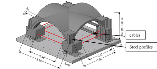
Figure 2. Setup of the unstrengthened model (UNS) and strengthened model (SM).

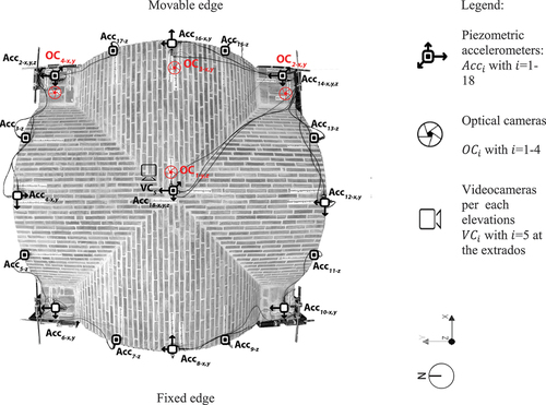
Figure 3. Time histories of the target input signals of AQA earthquake: accelerations, velocities, and displacements.

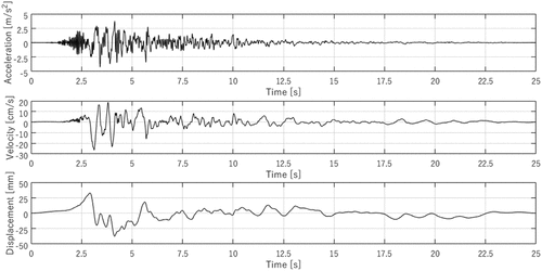
Table 1. List of tests carried out on the unstrengthened test specimen: dynamic identification tests (DIT) and shaking table tests (ST).

ID	Denomination	Input direction	Description
1	DIT-0-UNS-Y	North-South	Dynamic identification test of the undamaged vault
2	DIT-0-UNS-X	East-West
3	ST-UNS-10%	North-South	Seismic test with amplitude equal to 10% of AQA eq.
4	ST-UNS-25%	North-South	Seismic test with amplitude equal to 25% of AQA eq.
5	DIT-1-UNS-Y	North-South	Dynamic identification after seismic test at the 25%
6	DIT-1-UNS-X	East-West
7	ST-UNS-50%	North-South	Seismic test with amplitude equal to 50% of AQA eq.
8	DIT-2-UNS-Y	North-South	Dynamic identification after seismic test at the 50%
9	DIT-2-UNS-X	East-West
10	ST-UNS-75%	North-South	Seismic test with amplitude equal to 75% of AQA eq.
11	DIT-3-UNS-Y	North-South	Dynamic identification after seismic test at the 75%
12	DIT-3-UNS-X	East-West

Table 2. List of tests carried out on the strengthened test specimen: dynamic identification tests (DIT) and shaking table tests (ST).

ID	Denomination	Input direction	Description
1	DIT-0-SM-Y	North-South	Dynamic identification test of repaired and strengthened vault
2	DIT-0-SM-X	East-West
3	ST-SM-25%	North-South	Seismic test with amplitude equal to 25% of AQA eq.
4	DIT-1-SM-Y	North-South	Dynamic identification after seismic test at the 25%
5	DIT-1-SM-X	East-West
6	ST-SM-50%	North-South	Seismic test with amplitude equal to 50% of AQA eq.
7	DIT-2-SM-Y	North-South	Dynamic identification after seismic test at the 50%
8	DIT-2-SM-X	East-West
9	ST-SM-75%	North-South	Seismic test with amplitude equal to 75% of AQA eq.
10	DIT-3-SM-Y	North-South	Dynamic identification after seismic test at the 75%
11	DIT-3-SM-X	East-West
12	ST-SM-100%	North-South	Seismic test with amplitude equal to 100% of AQA eq.
13	DIT-4-SM-Y	North-South	Dynamic identification after seismic test at the 100%
14	DIT-4-SM-X	East-West
15	ST-SM-125%	North-South	Seismic test with amplitude equal to 125% of AQA eq.
16	DIT-5-SM-Y	North-South	Dynamic identification after seismic test at the 125%
17	DIT-5-SM-X	East-West
18	ST-SM-150%	North-South	Seismic test with amplitude equal to 150% of AQA eq.
19	DIT-6-SM-Y	North-South	Dynamic identification after seismic test at the 150%
20	DIT-6-SM-X	East-West

Figure 4. FEM‒UNS macro-model of the full-scale vault in DIANA environment: (a) geometry, (b) mesh of the model.

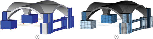
Table 3. Element types of the numerical FEM‒UNS and FEM – SM models built in DIANA 10.5 (2022).

Material	Type of element	Denomination
Masonry	Hexahedron solid element (CHX60)	Fixed piers
		Shell and filling
		Supports
Steel		Steel masses
		Steel profiles
		Steel frame
Steel	Enhanced truss element, straight (L6TRU)	Three couples of steel cables
Steel	Embedded bar in solid element	Steel connectors inside the fixed piers
	Interface element (CQ48I)	Boundary interface below the steel masses

Figure 5. Constitutive laws used in the FEM–UNS and FEM–SM models: (a) non-linear hysteretic behaviour of masonry elements, (c) Mohr–coulomb criterion for sliding interface.

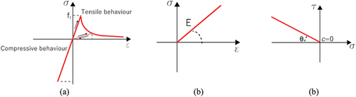
Figure 6. Strengthened FEM‒SM macro-model of the full-scale vault in DIANA 10.5 (2022) environment: (a) shell element (CQ40S) for the Geocalce F, (b) embedded grid to simulate geosteel grid 200.

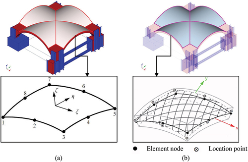
Figure 7. Grout injections modelled in the strengthened FEM‒SM model in DIANA 10.5 (2022): (a) damaged intrados at the end of the ST–UNS–75%, (b) solid elements to simulate injections (intrados and north elevation).

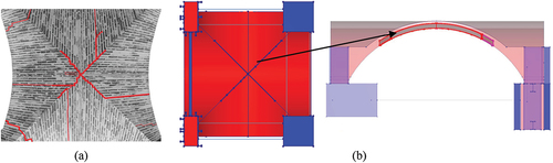
Table 4. Mechanical properties for the TRM system adopted in the numerical FEM‒SM (DIANA 10.5 2022.).

Material	Young’s modulus [GPa]	Density [kg/$m^3$]	Distributed mass [g/$m^2$]	Thickness [mm]
Grid Geosteel 200	62.0		200	10 mm
Mortar Geocalce F	12.5	1800	✗
Mortar Geocalce FL	7.81	1600		✗

Figure 8. Geometry of the DEM model in 3DEC 7.0 environment.

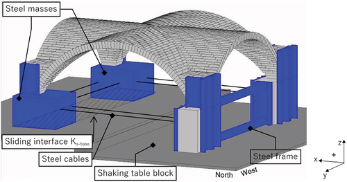
Figure 9. List of joints contact of the DEM model in 3DEC 7.0 environment.

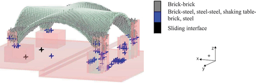
Figure 10. Contacts behaviour in the DEM model: (a) elastic joint model between brick-steel, shaking table-brick, shaking table-steel and steel-steel, (b) Mohr–coulomb criterion between brick-brick in the normal direction, (c) Mohr–coulomb criterion between brick-brick in the tangential direction.

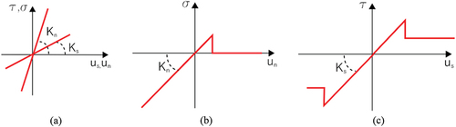
Figure 11. Failure surface implemented for Mohr–coulomb (MC) and combined material behaviour of Mohr–coulomb (MC‒CM). Adapted by Pulatsu (2023).

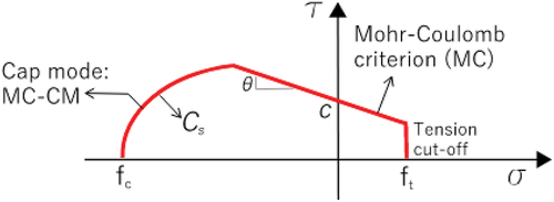
Figure 12. Mode shapes of the first modes of the specimens (UNS and SM) and numerical models: (a) DIT‒0–UNS–Y test, (b) first mode obtained from eigenvalue analysis for FEM‒UNS model, (c) DIT‒0–SM–Y test; (d) first mode obtained from eigenvalue analysis for FEM‒SM model.

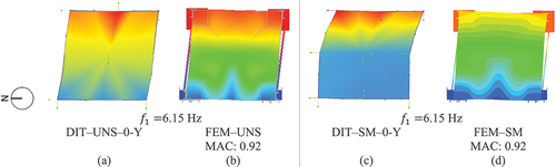
Table 5. Final properties after the calibration for FEM‒UNS and FEM‒SM models. $\ast$Calibrated properties.

	Linear properties
	Masonry (shell and infill)	Masonry (fixed piers)	Geocalce F	Geocalce FL	Steel elements
Young’s modulus [GPa]	0.96 (FEM‒UNS) 0.93 (FEM‒SM)	2.22	12.54	7.81	210.00
Mass density [kg/$m^3$]	2260	2260	1800	1600	7800
Poisson’s ratio	0.20	0.20	0.14	0.20	0.30
	Non-linear properties: TSCR material behaviour
	Masonry	Masonry
	(shell and infill)	(fixed piers)	Geocalce F	Geocalce FL	✗
	Exponential
Tensile strength [MPa]	0.1	0.30	1.3	0.8

Figure 13. Comparison of frequency response functions obtained from the numerical modelling and the dynamic identification tests. (DIT‒0–UNS–Y, red dashed line) and the numerical model (DEM‒UNS, black solid line).

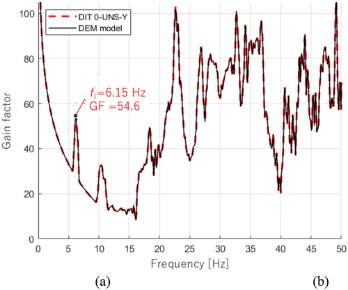
Table 6. Final properties of joints after the calibration for classic Mohr–Coulomb criterion in DEM‒UNS model. $\ast$Calibrated properties.

Joints	Normal stiffness $k_n$ [MPa/mm]	Shear stiffness $K_{\zeta }$ [MPa/mm]	Friction angle $\mathit{\theta }$ [°]	Dilatancy angle $\mathit{\psi }$ [rad]
Steel masses – shaking table (base)	20.0$\ast$	≈0$\ast$	2	null
Bricks – bricks	16.3$\ast$	6.5$\ast$	38

Figure 14. DEM calibration: (a) MAC matrix, (b) first mode shape between DIT (red) and DEM‒UNS (blue) model performing vibration analysis.

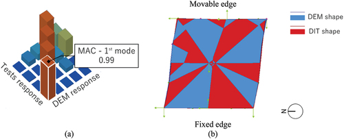
Table 7. List of analyses carried out on the unstrengthened and strengthened numerical models.

Denomination	PGA [m/${\mathrm{s}}^2$]	PGV [cm/s]	PGD [mm]	Shaking table tests	DEM‒UNS	FEM‒UNS
Unstrengthened
ST–UNS–25%	1.37	6.22	3.76	✓	✓ (In series)	✓
ST–UNS–50%	2.58	12.17	8.57			✓
ST–UNS–75%	3.62	18.17	17.57			✓
ST–UNS–100%	4.47	24.20	24.47	✗	✓	✗
Denomination	PGA [m/s^2]	PGV [cm/s]	PGD [mm]	Shaking table tests	DEM	FEM‒SM
Strengthened
ST–SM–150%	7.27	35.65	54.60	✓	✗	✓

Figure 15. Viscous damping of the numerical models.

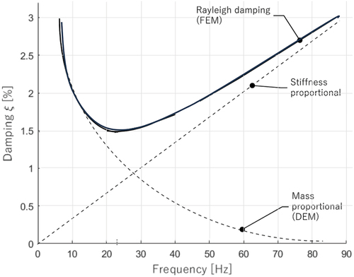
Figure 16. Evolution of cracks at the extrados: (a) ST–UNS–75, (b) deformed shapes of DEM‒UNS model (deformation factor: 100), (c) strains distribution in FEM‒UNS model.

Table 8. Peak values and root mean square of displacements (RMSD) and average errors between the results measured by $\mathit{O}{C}_{1,2,3,4}$ for each seismic test of the unstrengthened specimen and obtained by DEM‒UNS and FEM‒UNS models.

Sequence	$\mathit{O}{C}_1$ [mm]		$\mathrm{O}{\mathbf{C}}_2$ [mm]		$\mathrm{O}{\mathbf{C}}_3$ [mm]		$\mathrm{O}{\mathbf{C}}_4$ [mm]
	NS	Vertical	WE	NS	WE	NS	WE	NS
ST‒UNS‒75%	30.72	−10.64	4.40	52.51	5.08	32.80	7.77	32.05
FEM‒UNS‒75%	32.09	−8.51	1.13	36.3	1.08	36.56	0.98	37.09
DEM‒UNS‒75% with MC	22.23	−4.19	9.10	19.78	1.64	19.88	5.04	19.69
DEM‒UNS‒75% with MC‒CM	23.70	−3.45	0.74	22.61	2.51	23.50	0.63	26.60
	Average error $\bar{\epsilon }$ [%] (All the analyses: 25%, 50%, 75%), all $\mathbf{O}{\mathbf{C}}_{\mathbf{i}}$, NS direction)
			FEM‒UNS		DEM‒UNS with MC		DEM‒UNS with MC‒CM
	Peak values		14.45		41.95		30.06
	RMSD		16.57		24.12		18.92
	Average error $\bar{\epsilon }$ [%] (All the analyses: 25%,50%,75%), $\mathrm{O}{\mathrm{C}}_2$ discarded, NS direction)
			FEM‒UNS		DEM‒UNS with MC		DEM‒UNS with MC‒CM
	Peak values		12.53		35.37		21.57
	RMSD		7.60		15.55		10.00

Figure 17. Rmsds in the longitudinal direction: (a) $\mathrm{O}{\mathrm{C}}_1$, $\mathrm{O}{\mathrm{C}}_3$, $\mathrm{O}{\mathrm{C}}_4$, (b) $\mathrm{O}{\mathrm{C}}_2$.

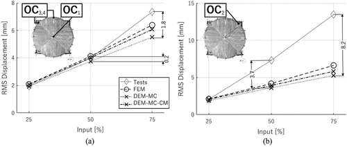
Figure 18. Comparison of the displacement profiles between experiments and numerical responses.

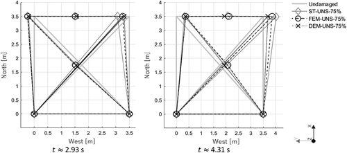
Figure 19. Damage map for: (a) ST–SM–150%, (b) principal strains distribution in FEM‒SM model.

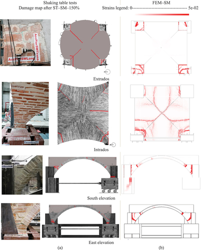
Figure 20. In-plane deformation profiles of the strengthened configuration for the ST–SM–150% when all the optical cameras measure the maximum displacements. Deformation factor: 10.

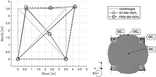
Table 9. Peak values and root mean square (RMSD) of displacements and average errors obtained from $\mathrm{O}{\mathrm{C}}_{1,2,3,4}$ of the ST — SM–150% and the FEM‒SM model.

Sequence	$\mathit{O}{C}_1$ [mm]		$\mathit{O}{C}_2$ [mm]		$\mathit{O}{C}_3$ [mm]		$\mathit{O}{C}_4$ [mm]
	NS	Vertical	WE	NS	WE	NS	WE	NS
ST–SM–150%	56.03	12.80	42.81	63.48	15.80	64.68	12.77	62.17
FEM‒SM–150%	54.70	11.43	13.51	67.02	5.19	62.26	9.35	59.51
	Average error (all $\mathrm{O}{\mathrm{C}}_{\mathrm{i}}$ in NS direction) $\bar{\epsilon }$ [%]
	FEM‒SM
	Peak values				1.2%
	RMSD				6.4%

DIANA 10.5. 2022. Finite element modelling software. Delft, Netherlands.

 Google Scholar

Pulatsu, B. 2023. Coupled elasto-softening contact models in DEM to predict the in-plane response of masonry walls. Computational Particle Mechanics 10 (6):1759–70. doi:10.1007/s40571-023-00586-x.

 Web of Science ®Google Scholar