‘The Equator–Pole grid system’: an overset grid system for the sphere, with an optimal uniformity property

Figures & data

Fig. 1. The grid system for a hemisphere, with N= 40 points around the equator, and without overlapping.

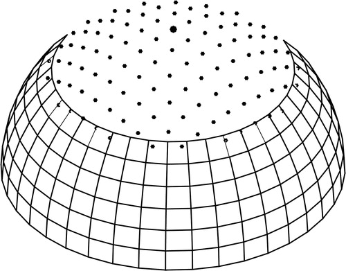
Fig. 2. Orthogonally projected grid system on the equatorial plane, with overlapping corresponding to the centred 4th order method, and with N= 40.

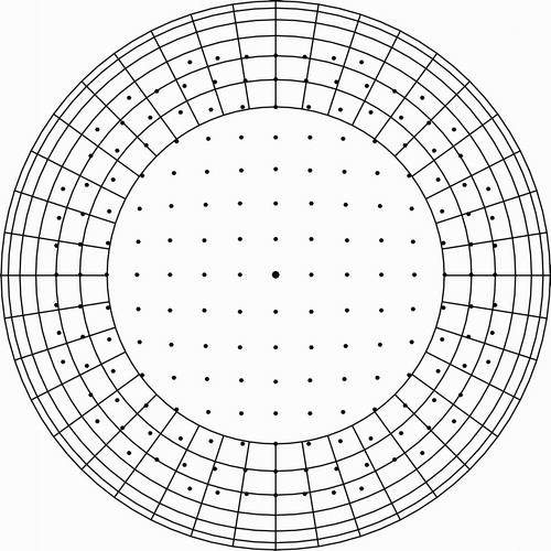
Table 5. The Rossby–Haurwitz wave: Relative changes of the total mass and energy.

$re{l}_{\mathit{\text{mass}}}(1:7)$	1.27e − 7	2.43e − 7	2.59e − 7	2.94e − 7	1.55e − 7	−1.01e − 7	−3.31e − 7
$re{l}_{\mathit{\text{mass}}}(8:14)$	−3.59e − 7	−2.92e − 7	−1.35e − 7	2.13e − 8	9.88e − 8	1.32e − 8	−1.81e − 7
$re{l}_{\mathit{\text{energy}}}(1:7)$	4.24e − 4	1.70e − 3	3.32e − 3	4.47e − 3	5.01e − 3	5.46e − 3	5.70e − 3
$re{l}_{\mathit{\text{energy}}}(8:14)$	5.67e − 3	5.70e − 3	5.56e − 3	5.16e − 3	5.12e − 3	5.34e − 3	5.15e − 3

N = 360, 2p = 4, s = 2, c = 1.7e − 5, $\Delta t=120$s, Time =14 days.

Table 3. Normalized errors for steady state geostrophic flow.

α	${10}^8·c$	2p	s	stc, ${\ell }_{\infty }(\Psi )$	stc,  ${\ell }_2(\Psi )$	${10}^8·c$	mstc,  ${\ell }_{\infty }(\Psi )$	mstc,  ${\ell }_2(\Psi )$
0	2.5	4	2	7.4896e − 8	2.7333e − 8	2.0	2.3393e − 8	1.4434e − 8
45	94.5	4	2	4.5811e − 6	7.1803e − 7	15.0	9.8324e − 7	1.3341e − 7
90	3.5	4	2	3.3136e − 7	1.4239e − 7	3.5	3.3416e − 7	1.5007e − 7
0	0	6	3	3.2131e − 10	1.0983e − 10	0	1.7475e − 11	8.0196e − 12
45	0	6	3	4.9529e − 8	2.4985e − 9	0	3.7105e − 10	1.0249e − 10
90	0	6	3	5.7385e − 10	2.2245e − 10	0	4.1246e − 10	2.0270e − 10

N = 240, $\Delta t=300$s, Time =5 days, stc: = stereographic coord. and mstc: = modified stereographic coord.

Table 2. Normalized errors for solid rotation of the Cosine bell.

α	${10}^8·c$	2p	s	$\min H$	$\max H$	${\ell }_{\infty }(H)$	${\ell }_2(H)$
90	98.5	4	2	−7.4455	9.9906e + 2	7.4455e − 3	6.5382e − 3
87	101.5	4	2	−7.4175	9.9904e + 2	7.4175e − 3	6.5323e − 3
45	43.0	4	2	−6.2911	9.9758e + 2	6.2919e − 3	7.2938e − 3
90	98.5	4	3	−7.4441	9.9907e + 2	7.4452e − 3	6.5374e − 3
87	102.0	4	3	−7.4151	9.9904e + 2	7.4169e − 3	6.5313e − 3
90	14.5	6	3	−2.7415	9.9958e + 2	2.7466e − 3	2.3972e − 3
87	12.0	6	3	−2.7398	9.9956e + 2	2.7844e − 3	2.5172e − 3
87	12.0	8	4	−1.6730	1.0000e + 3	1.6995e − 3	2.2057e − 3

N = 360, $\Delta t=600$s, Time =12 days, $\min {\ell }_{\infty }(H)$.

Fig. 3. Contour curves for smooth deformational flow: $\alpha ={45}^o$, N = 240, 2p = 4 and Time=12 days.

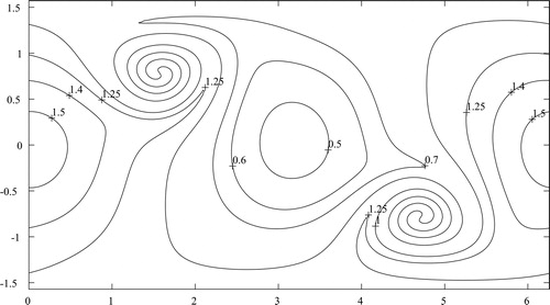
Table 1. Normalized errors for smooth deformational flow, stationary vortex.

α	${10}^8·c$	2p	s	$\min \Psi$	$\max \Psi$	${\ell }_{\infty }(\Psi )$	${\ell }_2(\Psi )$
0	1.0	4	2	0.46295	1.5370	4.9954e − 3	6.4872e − 4
45	3.5	4	2	0.46299	1.5370	4.9587e − 3	5.6236e − 4
90	1.6	4	2	0.46297	1.5370	7.5553e − 3	1.0074e − 3
0	0.25	6	3	0.46295	1.5370	1.1315e − 3	1.2714e − 4
45	0.35	6	3	0.46299	1.5370	1.1612e − 3	1.0952e − 4
90	0.45	6	3	0.46297	1.5370	2.1246e − 3	2.4623e − 4

N = 240, $\Delta t=400$s, Time =12 days.

Fig. 4. Absolute errors as function of lat–lon, with 2p = 6, N = 240 and $\Delta t=300$.

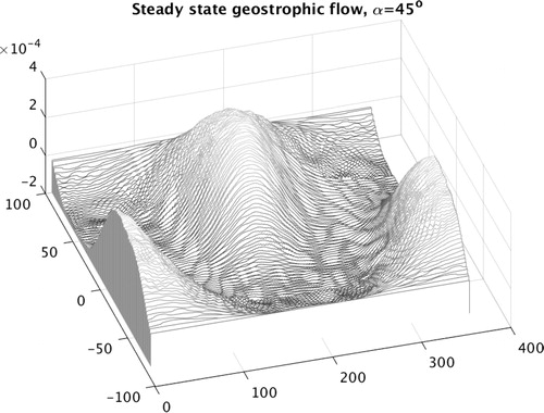
Fig. 5. Geostrophic flow with compact support, with $\alpha =60°$ and N= 240.

Table 4. Normalized errors for geostrophic flow with compact support.

α	${10}^8·c$	2p	s	$\min \Psi$	$\max \Psi$	${\ell }_{\infty }(\Psi )$	${\ell }_2(\Psi )$
0	7.0	4	2	2.0572e + 4	2.9401e + 4	4.4288e − 6	1.1233e − 6
60	10.5	4	2	2.0572e + 4	2.9401e + 4	2.0841e − 5	4.0558e − 6
0	0	6	3	2.0572e + 4	2.9401e + 4	7.5006e − 8	1.3479e − 8
60	0	6	3	2.0572e + 4	2.9401e + 4	2.8129e − 7	5.3725e − 8

N = 240, $\Delta t=300$s, Time =5 days.

Fig. 6. Absolute errors as function of lat–lon, with 2p = 6, N = 240 and $\Delta t=300$.

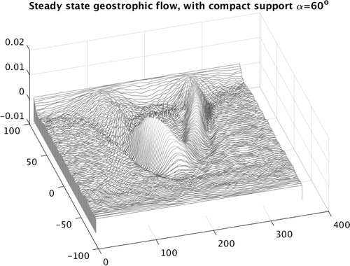
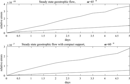
Fig. 7. Test problems no. 2 and 3 from Williamson et al. (1992). In each panel the lower curve correspond to ${\ell }_2(\Psi )$ and the upper to ${\ell }_{\infty }(\Psi )$. In all cases 2p = 6, N = 240 and $\Delta t=300$.

Williamson, D. L., Drake, J. B., Hack, J. J., Jakob, R. and Swarztrauber, P. N. 1992. A standard test set for numerical approximation to the shallow water equations in spherical geometry. J. Comput. Phys. 102, 211–224. doi:10.1016/S0021-9991(05)80016-6.

 Web of Science ®Google Scholar