
Figures & data
Figure 1. Flowchart of the study design. GEO, Gene Expression Omnibus; GSE, GEO Series; MM, multiple myeloma; DEGs, differentially expressed genes; WGCNA, weighted gene coexpression network analysis; GO, gene ontology; KEGG, Kyoto Encyclopedia of Genes and Genomes; PPI, protein–protein interaction; ROC curve, receiver operator characteristic curve; GSEA, gene set enrichment analysis.
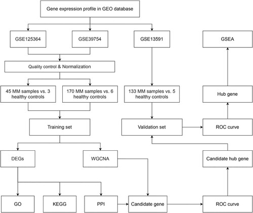
Figure 2. Screening of DEGs. (A) PCA shows that MM samples and healthy controls belong to different subgroups. (B) Volcano plot with cut-off criteria set to adjusted P-value < 0.05 and |log2FC| > 1. Red dots indicate upregulated genes, and blue dots indicate downregulated genes. Arrows indicate the location of the candidate hub genes. (C) Heatmap of the top 100 DEGs according to the values of |log2FC|. DEGs, differentially expressed genes; PCA, principal component analysis; MM, multiple myeloma; FC, fold change.
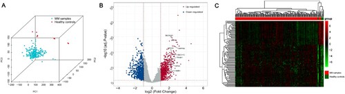
Figure 3. GO and KEGG pathway analysis of DEGs. (A-D) The bubble diagrams show the top 10 functional and pathway enrichment results with significant differences. (A) BP. (B) MF. (C) CC. (D) KEGG. GO, Gene Ontology; KEGG, Kyoto Encyclopedia of Genes and Genomes; DEGs, differentially expressed genes; BP, biological process; MF, molecular functions; CC, cellular components.
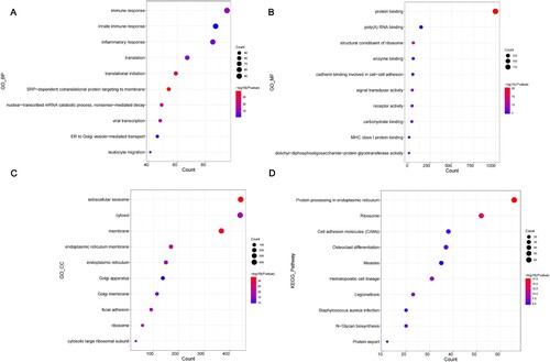
Figure 4. Candidate genes in the PPI network. (A) The PPI network of 1145 protein coding genes. (B) Venn diagram shows the shared genes based on 5 types of algorithms. PPI, protein–protein interaction.
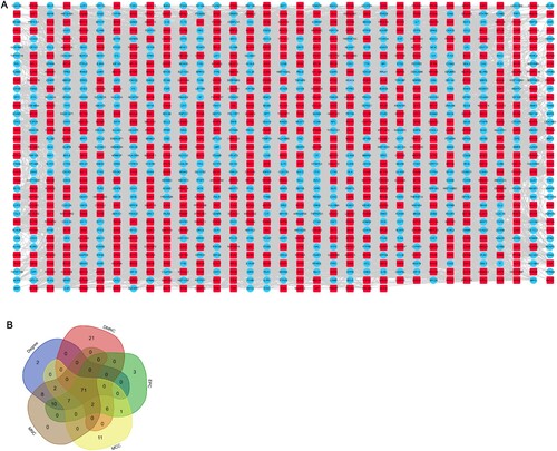
Figure 5. The process of WGCNA. (A) Sample clustering to detect outliers and the trait heatmap to display the sample traits. (B) Analysis of the network topology for various soft thresholding powers; the left panel shows the scale-free fit index (y-axis) as a function of the soft-thresholding power (x-axis); the right panel displays the mean connectivity (degree, y-axis) as a function of the soft-thresholding power (x-axis); the power was set as 15 for further analysis. (C) Clustering dendrograms for the 16 239 genes with dissimilarity based on the topological overlap together with the assigned module colors; twenty-six co-expression modules were constructed with various colors; the relationship between gene dendrogram and gene modules was up and down of the image. (D) The eigengene dendrogram and heatmap identify groups of correlated eigengenes termed meta-modules; the dendrogram indicated that the tan module was highly related to the MM; the heatmap in the panel shows the eigengene adjacency. (E) Visualizing 1 000 random genes from the network using a heatmap plot to depict the TOM among the genes in the analysis; the depth of the red color is positively correlated with the strength of the correlation between the pairs of modules on a linear scale; the gene dendrogram and module assignment are shown along the left side and the top. (F) Module-trait relationships; each row corresponds to a module eigengene, each column corresponds to a trait, and each cell consists of the corresponding correlation and P-value, which are color-coded by correlated according to the color legend. Among them, the tan module was the most relevant module to the MM. (G) Scatterplot of 209 genes in the tan module; the correlation and P-value are under the title. WGCNA, weighted gene coexpression network analysis; MM, multiple myeloma; TOM, topological overlap matrix.
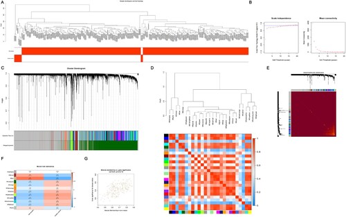
Figure 6. Identification and evaluation of candidate hub genes. (A) Venn diagram shows the shared candidate hub genes based on WGCNA and PPI analysis. (B) The interrelation between enriched pathways of candidate hub genes. The rhombus represents candidate hub genes; the circles represent enriched pathways. (C) ROC curves of candidate hub genes in diagnosing MM in the training set. Data are presented as cut-off values (sensitivity, specificity). WGCNA, weighted gene coexpression network analysis; MM, multiple myeloma; PPI, protein–protein interaction; ROC, receiver operator characteristic; AUC, area under the curve.
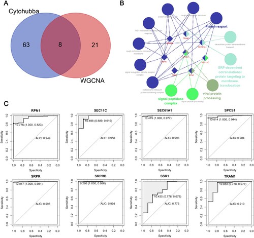
Figure 7. Validation of candidate hub genes. (A) Expression level of candidate hub genes in the validation set. (B) ROC curves of candidate hub genes in diagnosing MM in the validation set. (C) ROC curves of the RF model in diagnosing MM of the training set (left) and validation set (right). Data are presented as cut-off values (sensitivity, specificity). (D) DCA for the clinical practicability of the RF model of the training set (left) and validation set (right). ROC, receiver operator characteristic; AUC, area under the curve; MM, multiple myeloma; RF, random forest; DCA, decision curve analysis; *, P-value ≤ 0.05; ns, not significant.
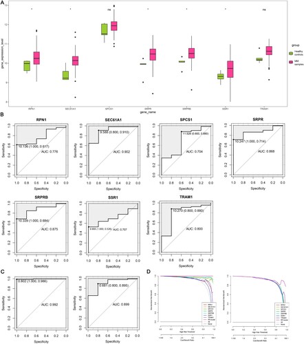
Table 1. GSEA of the hub genes (GO analysis).
Table 2. GSEA of the hub genes (KEGG pathway analysis).