Comparison of aircraft observations with ensemble forecast model results in terms of the microphysical characteristics of stratiform precipitation

Figures & data

Table 1. Summary of instruments and parameters used in this study.

Instrument	Manufacturer	Range	Resolution	Application
CIP	DMT	25–1550 μm	25 μm	Cloud droplets
HVPS	SPEC	150–8700 μm	150–750 μm	Precipitation particles
CPI	SPEC	10–2000 μm	2.3 μm	Images of cloud droplets, ice crystals, raindrops
LWC	Nevzorov	0–3 g m^−3		Liquid water content
TWC	Nevzorov	0–3 g m^−3		Total water content
AIMMS-20	DMT			Temperature, pressure, humidity, wind velocity

Table 2. Model configuration.

Member	Surface layer scheme	Planetary boundary layer physics scheme
C00	CLM4	YSU
C01	CLM4	MYNN2
C02	NOAH	YSU
C03	RUC	YSU
C04	NOAH	YSU
C05	CLM4	MYNN2
C06	NOAH	MYNN2
C07	RUC	MYNN2
C08	CLM4	YSU
C09	NOAH	YSU

Figure 1. Six-hour accumulated precipitation of (a) the control member (C00) and (b) the observation; six-hour accumulated precipitation (c) in the aircraft observation region of the control member (C00) and (d) in the flight track region of the observation. The red line represents the flight track of the aircraft. The black rectangle represents three regions: AB, CD, and EF. The black annotations in (c, d) are the times of the flight observation. The hourly 0.1° gridded precipitation dataset resulting from the fusion of China’s automated stations and CMORPH is used as the observation data.

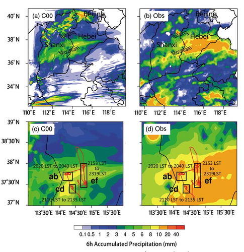
Figure 2. (a) Vertical distributions of LWC in region AB. The blue line represents the LWC from the control member (C00). The light gray line represents the LWC from the nine perturbation members (C01–C09). The red line is the ensemble average. The black line represents the result of the observation (average values of every 500 m) and the standard deviations at both ends. The green line represents the result of the observation (median values of every 500 m) and the standard deviations at both ends. (b) As in (a) but for IWC. (c) As in (a) but for ice and rain particle number concentration. (d) High-resolution particle image from CPI at different heights.

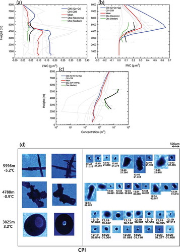
Figure 3. (a) Vertical distributions of LWC in region CD. The blue line represents the LWC from the control member (C00). The light gray line represents the LWC from the nine perturbation members (C01–C09). The red line is the ensemble average. The black line represents the result of the observation (average values of every 500 m) and the standard deviations at both ends. The green line represents the result of the observation (median values of every 500 m) and the standard deviations at both ends. (b) As in (a) but for IWC. (c) As in (a) but for ice and rain particle number concentration. (d) High-resolution particle image from CPI at different heights.

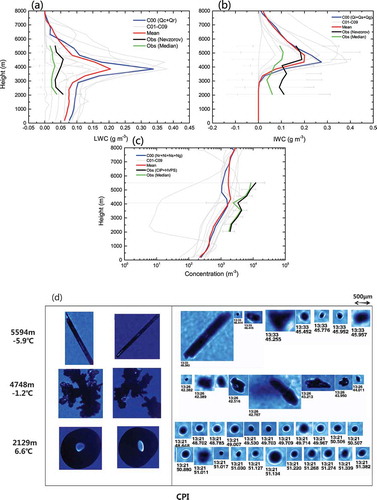
Figure 4. (a) Vertical distributions of LWC in region EF. The blue line represents the LWC from the control member (C00). The light gray line represents the LWC from the nine perturbation members (C01–C09). The red line is the ensemble average. The black line represents the result of the observation (average values at altitudes of 5600, 5100, 4800, 4300, 3600, 3000, 2400, and 2100 m) and the standard deviations at both ends. The green line represents the result of the observation (median values at altitudes of 5600, 5100, 4800, 4300, 3600, 3000, 2400, and 2100 m) and the standard deviations at both ends. (b) As in (a) but for IWC. (c) As in (a) but for ice and rain particle number concentration. (d) High-resolution particle image from CPI at different heights.

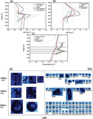
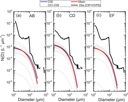
Figure 5. (a) Particle size distribution of raindrops for AB region (2400 m, 6.3°C). The blue line represents the control member (C00). The light gray line represents nine perturbation members (C01–C09). The red line represents the ensemble average. The black line represents the observation. (b) The same as (a), but for CD region. (c) The same as (a), but for EF region.