366
Views
21
CrossRef citations to date
0
Altmetric
Articles

Identification of materials in a hyperbolic annular fin for a given temperature requirement

Pages 213-233 | Received 19 Jun 2014, Accepted 06 Feb 2015, Published online: 03 Mar 2015

Figures & data

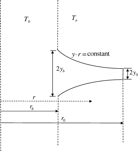
Figure 1. Geometry of the hyperbolic fin.

Figure 1. Geometry of the hyperbolic fin.

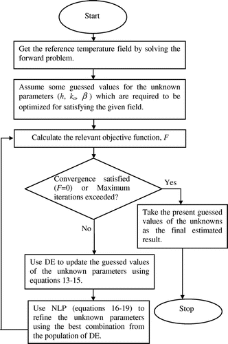
Figure 2. Flowchart of the inverse method.

Figure 2. Flowchart of the inverse method.

Table 1. Different values of parameters considered to be fixed during the inverse analysis.

Figure 3. Validation of the forward method for different non-dimensional thermo-physical parameters.
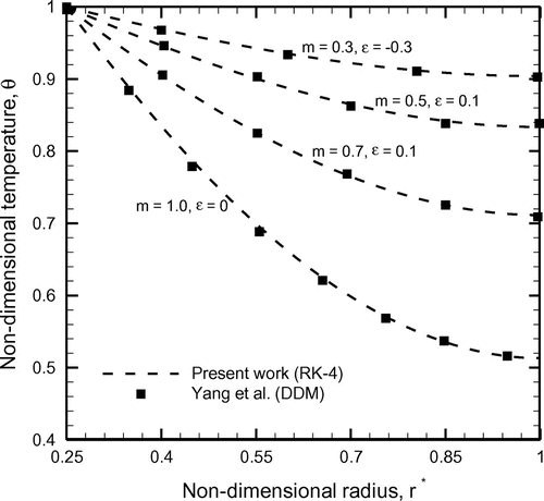
Figure 3. Validation of the forward method for different non-dimensional thermo-physical parameters.

Table 2. Estimated values of various unknowns for temperature field without measurement error, er = 0. (Forward non-dimensional parameters: m = 0.7, ε = 0.1 and rb* = 0.25.)

Figure 4. Variation of the objective function, F and unknown parameters (h, k, β) with number of iterations of hybrid algorithm; er = 0.
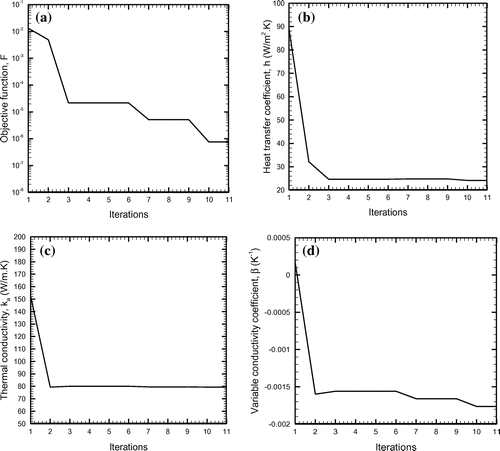
Figure 4. Variation of the objective function, F and unknown parameters (h, k, β) with number of iterations of hybrid algorithm; er = 0.

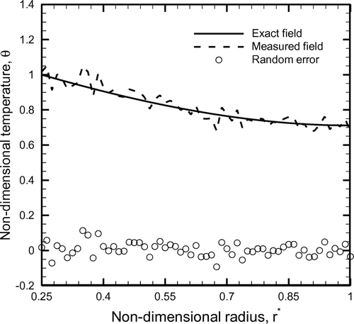
Figure 5. Comparison of the exact and measured temperature fields along with measurement error; m = 0.7, e = 0.1 and rb* = 0.25.

Figure 5. Comparison of the exact and measured temperature fields along with measurement error; m = 0.7, e = 0.1 and rb* = 0.25.

Table 3. Estimated values of various unknowns for temperature field with measurement error, er ≠ 0. (Forward non-dimensional parameters: m = 0.7, e = 0.1 and rb* = 0.25.)

Figure 6. Variation of the objective function, F and unknown parameters (h, k, β) with number of iterations of hybrid algorithm; er ≠ 0.
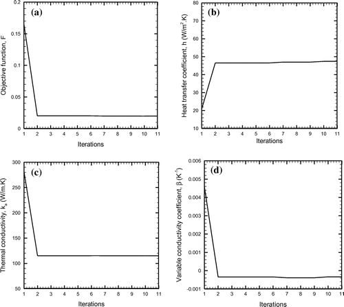
Figure 6. Variation of the objective function, F and unknown parameters (h, k, β) with number of iterations of hybrid algorithm; er ≠ 0.

Figure 7. Comparison of the exact and reconstructed temperature fields, (a) without involving measurement error, er = 0, (b) and (c) involving measurement error, er ≠ 0.
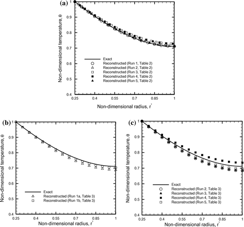
Figure 7. Comparison of the exact and reconstructed temperature fields, (a) without involving measurement error, er = 0, (b) and (c) involving measurement error, er ≠ 0.

Figure 8. Comparison of the residuals between the exact and the reconstructed temperature fields, (a) without involving measurement error, er = 0 and (b) involving measurement error, er ≠ 0.
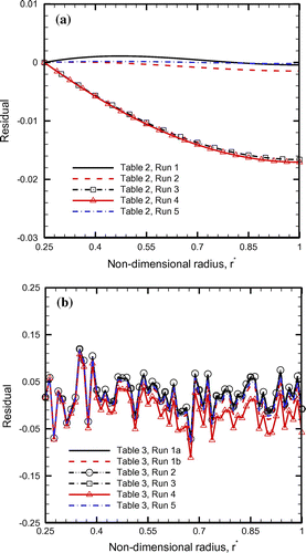
Figure 8. Comparison of the residuals between the exact and the reconstructed temperature fields, (a) without involving measurement error, er = 0 and (b) involving measurement error, er ≠ 0.

Figure 9. Comparison of the exact and the reconstructed temperature fields for different measurement points.
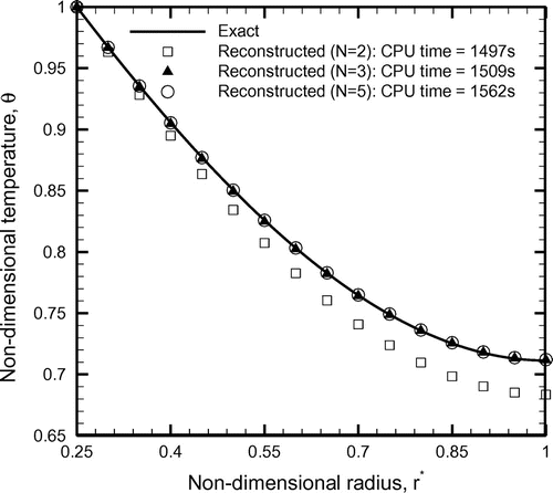
Figure 9. Comparison of the exact and the reconstructed temperature fields for different measurement points.
Reprints and Corporate Permissions

Please note: Selecting permissions does not provide access to the full text of the article, please see our help page How do I view content?

To request a reprint or corporate permissions for this article, please click on the relevant link below:

Academic Permissions

Please note: Selecting permissions does not provide access to the full text of the article, please see our help page How do I view content?

Obtain permissions instantly via Rightslink by clicking on the button below:

If you are unable to obtain permissions via Rightslink, please complete and submit this Permissions form. For more information, please visit our Permissions help page.