504
Views
12
CrossRef citations to date
0
Altmetric
Articles

Inverse problem in the hyperthermia therapy of cancer with laser heating and plasmonic nanoparticles

, &
Pages 608-631 | Received 08 Nov 2015, Accepted 03 Apr 2016, Published online: 13 May 2016

Figures & data

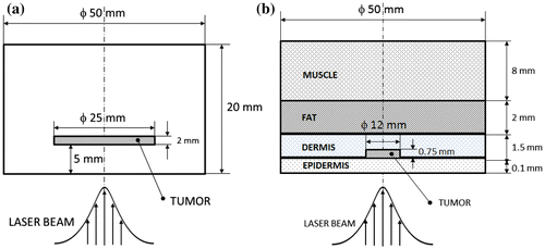
Figure 1. Sketches of the cases examined in this work: (a) soft tissue phantom; (b) skin model.

Figure 1. Sketches of the cases examined in this work: (a) soft tissue phantom; (b) skin model.

Table 1. Auxiliary sampling importance resampling (ASIR) algorithm.[Citation28,29]

Table 2. Thermophysical and optical properties of the PVCP phantom.[Citation32,44,45]

Table 3. Optical properties of region loaded with gold nanorods.

Figure 2. Exact and estimated temperature distribution at selected times with N = 100 particles and with N = 250 particles.
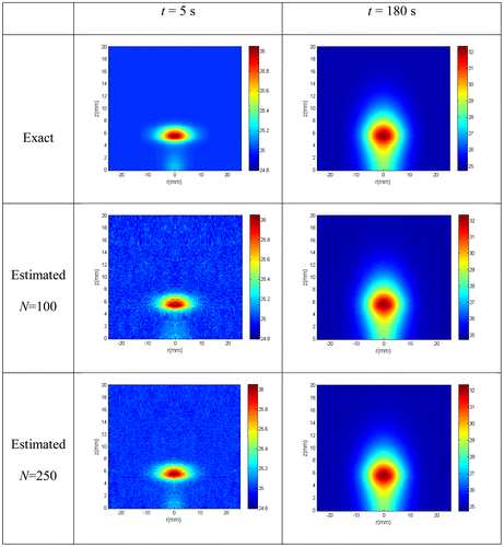
Figure 2. Exact and estimated temperature distribution at selected times with N = 100 particles and with N = 250 particles.

Figure 3. Estimated and exact temperature distribution at t = 180 s: (Left) along the radius for a line at z = 6 mm of the inclusion with N = 100 particles (a) and N = 250 particles (b); (Right) along the centerline with N = 100 particles (c) and N = 250 particles (d).
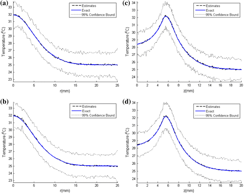
Figure 3. Estimated and exact temperature distribution at t = 180 s: (Left) along the radius for a line at z = 6 mm of the inclusion with N = 100 particles (a) and N = 250 particles (b); (Right) along the centerline with N = 100 particles (c) and N = 250 particles (d).

Figure 4. Comparison of the estimated and exact transient temperature variations with the temperature measurements at the sensor position (r = 2 mm, z = 6 mm): (a) N = 100 particles; (b) N = 250 particles.

Figure 4. Comparison of the estimated and exact transient temperature variations with the temperature measurements at the sensor position (r = 2 mm, z = 6 mm): (a) N = 100 particles; (b) N = 250 particles.

Figure 5. Estimated and exact transient temperature variations: (Left) at (r = 15 mm, z = 6 mm) with N = 100 particles (a) and N = 250 particles (b); (Right) at (r = 0 mm, z = 10 mm) with N = 100 particles (c) and N = 250 particles (d).
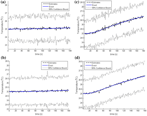
Figure 5. Estimated and exact transient temperature variations: (Left) at (r = 15 mm, z = 6 mm) with N = 100 particles (a) and N = 250 particles (b); (Right) at (r = 0 mm, z = 10 mm) with N = 100 particles (c) and N = 250 particles (d).

Figure 6. (a) Exact fluence rate distribution; (b) Fluence rate distribution estimated with N = 250 particles.
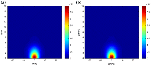
Figure 6. (a) Exact fluence rate distribution; (b) Fluence rate distribution estimated with N = 250 particles.

Table 4. Thermophysical and optical properties of tissues.[Citation33,34,47]

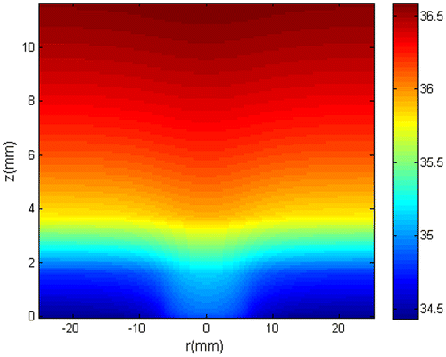
Figure 7. Initial temperature distribution.

Figure 7. Initial temperature distribution.

Table 5. Optical properties of the tumour-containing gold nanorods.

Figure 8. Exact and estimated temperature distribution at selected times with N = 100 particles and N = 250 particles.
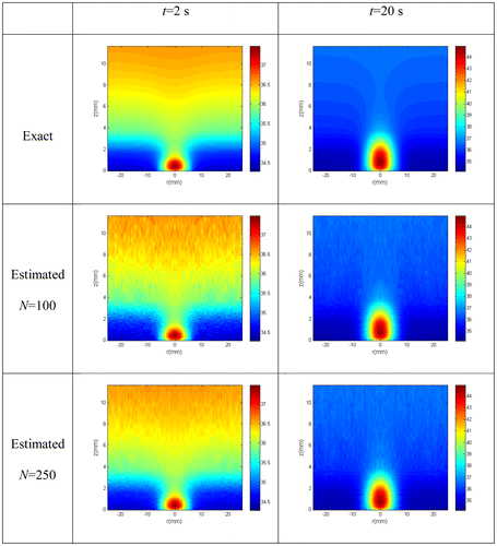
Figure 8. Exact and estimated temperature distribution at selected times with N = 100 particles and N = 250 particles.

Figure 9. Estimated and exact temperature distribution at t = 20 s: (Left) along the radius for a line at z = 0.7 mm with N = 100 particles (a) and N = 250 particles (b); (Right) along the centerline with N = 100 particles (c) and N = 250 particles (d).
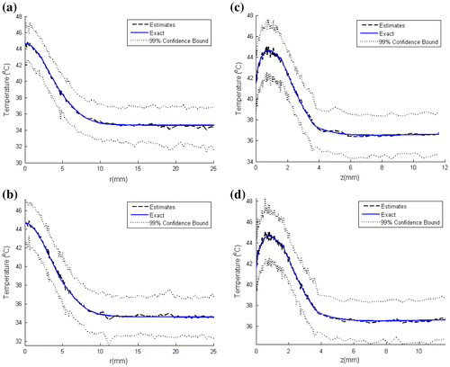
Figure 9. Estimated and exact temperature distribution at t = 20 s: (Left) along the radius for a line at z = 0.7 mm with N = 100 particles (a) and N = 250 particles (b); (Right) along the centerline with N = 100 particles (c) and N = 250 particles (d).

Figure 10. Comparison of the estimated and exact transient temperature variations with the temperature measurements at the sensor position (r = 0.5 mm, z = 0.7 mm): N = 100 particles (a); N = 250 particles (b).
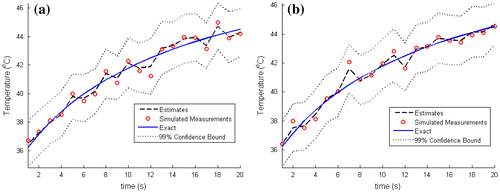
Figure 10. Comparison of the estimated and exact transient temperature variations with the temperature measurements at the sensor position (r = 0.5 mm, z = 0.7 mm): N = 100 particles (a); N = 250 particles (b).

Figure 11. Estimated and exact transient temperature variations: (Left) at (r = 6 mm, z = 0.7 mm) with N = 100 particles (a) and N = 250 particles (b); (Right) at (r = 0 mm, z = 3 mm) with N = 100 particles (c) and N = 250 particles (d).
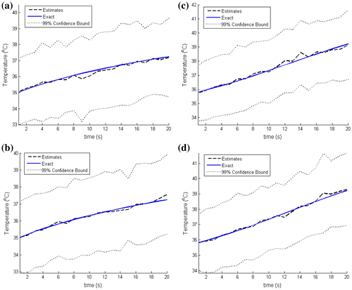
Figure 11. Estimated and exact transient temperature variations: (Left) at (r = 6 mm, z = 0.7 mm) with N = 100 particles (a) and N = 250 particles (b); (Right) at (r = 0 mm, z = 3 mm) with N = 100 particles (c) and N = 250 particles (d).

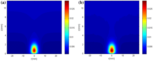
Figure 12. (a) Exact fluence rate distribution; (b) Fluence rate distribution estimated with N = 250 particles.
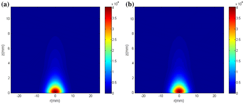
Figure 12. (a) Exact fluence rate distribution; (b) Fluence rate distribution estimated with N = 250 particles.

Figure 13. (a) Exact thermal damage distribution; (b) Estimated thermal damage distribution with N = 250 particles.

Figure 13. (a) Exact thermal damage distribution; (b) Estimated thermal damage distribution with N = 250 particles.

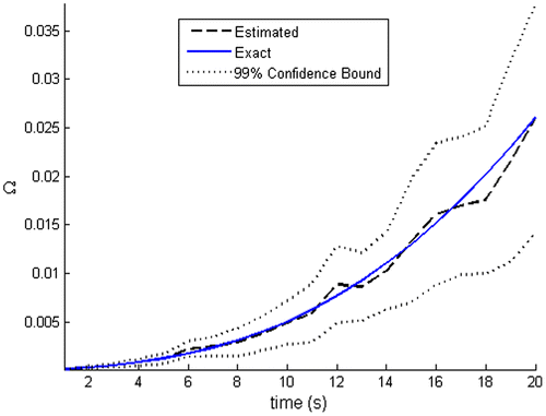
Figure 14. Comparison of the transient variation of the thermal damage calculated with the exact and estimated temperatures at the position (r = 0.5 mm, z = 0.7 mm).

Figure 14. Comparison of the transient variation of the thermal damage calculated with the exact and estimated temperatures at the position (r = 0.5 mm, z = 0.7 mm).

Reprints and Corporate Permissions

Please note: Selecting permissions does not provide access to the full text of the article, please see our help page How do I view content?

To request a reprint or corporate permissions for this article, please click on the relevant link below:

Academic Permissions

Please note: Selecting permissions does not provide access to the full text of the article, please see our help page How do I view content?

Obtain permissions instantly via Rightslink by clicking on the button below:

If you are unable to obtain permissions via Rightslink, please complete and submit this Permissions form. For more information, please visit our Permissions help page.