A complex elastographic hyperbolic solver (CEHS) to recover frequency dependent complex shear moduli in viscoelastic models utilizing one or more displacement data-sets

Figures & data

Figure 1. Diagrams of viscoelastic models: (a) Kelvin–Voigt fractional derivative model; (b) Spring-pot model; (c) Standard linear solid model.

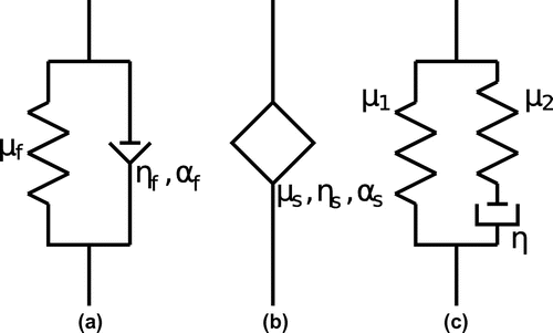
Figure 2. Exact value of complex modulus at frequency 25 Hz(KVFD), 20 Hz(SP) and 12.5 Hz(SLS): (a) real part, KVFD model; (b) real part, SP model; (c) real part, SLS model; (d) imaginary part, KVFD model; (e) imaginary part, SP model; (f) imaginary part, SLS model. Notice that in all cases, the imaginary part is smaller than the real part. The units for the images are KPa.

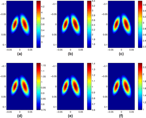
Figure 3. Recovery from two data-sets: (a) real part, KVFD model; (b) real part, SP model; (c) real part, SLS model; (d) imaginary part, KVFD model; (e) imaginary part, SP model; (f) imaginary part, SLS model. The units for the images are KPa.

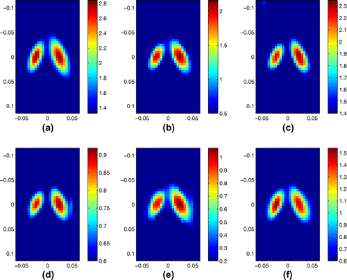
Figure 4. Recovery from algebraic inversion: (a) real part, KVFD model; (b) imaginary part, KVFD model; (c) absolute value of the error of real part, KVFD Model; (d) absolute value of the error of imaginary part, KVFD Model; (e) real part, SP Model; (f) imaginary part, SP model; (g) absolute value of the error of real part, SP model; (h) absolute value of the error of imaginary part, SP Model; (i) real part, SLS Model; (j) imaginary part, SLS model; (k) absolute value of the error of real part, SLS model; (l) absolute value of the error of imaginary part, SLS Model. The units for the images are KPa.

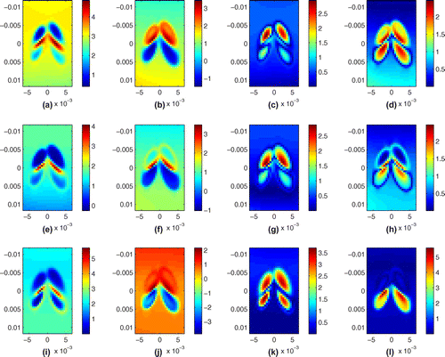
Figure 5. Recovery from two data-sets: (a) real part, KVFD model; (b) real part, SP model; (c) real-part SLS model; (d) imaginary part, KVFD model; (e) imaginary part, SP model; (f) imaginary part, SLS model. The units for the images are KPa.

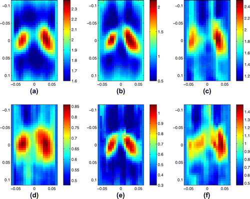
Figure 6. Region of Interest (ROI) in the experimental set-up. The depth is 40 mm and width is 18 mm. The focal depth is 25 mm. The ROI is made up of 31 vectors or locations where data are collected.

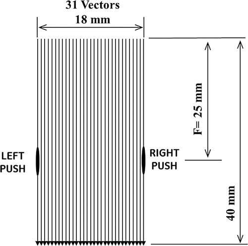
Figure 7. Graphic display of scan sequence at each location. Horizontal axis is time.

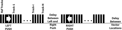
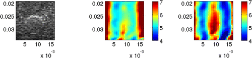
Figure 8. Recovery from phantom data: (a) B-mode image; (b) real part, p.d.e. solver at 243.75 Hz; (c) real part, p.d.e. solver at 268.75 Hz; (d) real part, Algebraic Inversion at 268.75 Hz; (e) imaginary part, p.d.e. solver at 243.75 Hz; (f) imaginary part, p.d.e. solver at 268.75 Hz; (g) imaginary part, Algebraic Inversion at 268.75 Hz. The units for the shear modulus images are KPa.

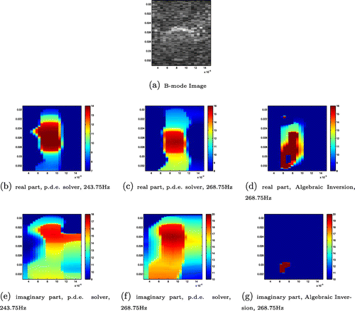
Table 1. Fitted viscoleastic parameters.

KVFD model	${\mathit{\mu }}_f$	${\mathit{\eta }}_f$	${\mathit{\alpha }}_f$
Value	10.03 KPa	0.0.03 KPa s	0.84
FD model	${\mathit{\mu }}_s$	${\mathit{\tau }}_s$	${\mathit{\alpha }}_s$
Value	5.18 KPa	0.01s	0.50
SLS model	${\mathit{\mu }}_1$	${\mathit{\mu }}_2$	$\mathit{\tau }$
Value	11.07 KPa	77.13 KPa	0.0001 s

Figure 9. Average value inside the inclusion and corresponding fitted curves from all three viscoelastic models: (a) real part; (b) imaginary part; red curve is KVFD model, black curve is SP Model, green curve is Zener Model, dotted red line with green blocks is the averaged value inside the inclusion.

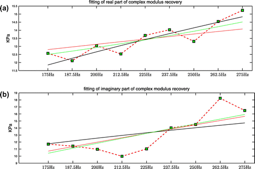
Figure 10. Wave speed calculated from average complex modulus values in the inclusion, along with wave speed calculated from best-fit complex modulus curves.

Figure 11. B-mode image (left) and recovered shear wave speed images using repetition frequencies 277.7 Hz (left) and 416.6 Hz (right), corresponding to time shifts of $N=12$ time steps and $N=8$ time steps, respectively. The units on the horizontal and vertical axes are meters and the units on the colourbar are m/s.