A numerical scheme based on discrete mollification method using Bernstein basis polynomials for solving the inverse one-dimensional Stefan problem

Figures & data

Figure 1. Domain representation of the one-phase Stefan problem.

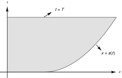
Table 1. RMS and CPU time(s) for $g(t)$ in Example 6.1.

ϵ	N	RMS for new technique	RMS for old technique	CPU time(s) for new technique	CPU time(s) for old technique
0.001	100	0.000423465	0.000479141	0.280802	6.02164
0.001	150	0.000393147	0.000478458	0.608126	9.00126
0.001	200	0.000373714	0.000430193	0.998406	12.2773

Table 2. RMS for $g(t)$ in Example 6.2.

ϵ	N	RMS for new technique	RMS for old technique [25]
0.00	128	0.00032	0.00049
0.05	128	0.01032	0.01555
0.10	128	0.01855	0.03249
0.00	256	0.00010	0.00014
0.05	256	0.00915	0.01398
0.10	256	0.01694	0.03773

Table

N	number of time partitions of the grid,
k	time step (the time nodes are $t_n=nk$ for $n=0,1,\dots ,N$),
$M_0$	number of the space partitions for interval $[0,s(t_0)]$,
h	space step with $h=\mathrm{\Delta }x=s(t_0)/M_0$,
$M_n$	integer part of the space partitions for interval $[0,s(t_n)],n=1,\dots ,N$,
	such that $s(t_n)=(M_n+{\theta }_n)h$ and $0\le {\theta }_n<1$,
$U_j^n$	discrete computed approximation of $w(x_j,t_n)$,
$Q_j^n$	discrete computed approximation of $w_x(x_j,t_n)$,
$W_j^n$	discrete computed approximation of $w_t(x_j,t_n)$.

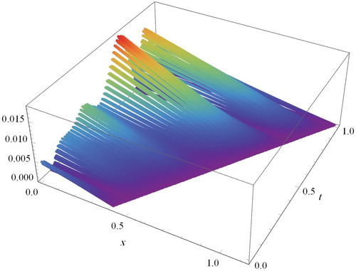
Figure 2. The unknown $U_{M_n}^n$ at the $(M_n,n)$th mesh point calculated in step 3 for $n=1,\dots ,N$ with N = 3 and $M_0=3$, where $M_n=[s(t_n)/h]$.

Figure 3. Graphs of exact and regularized data functions for $g(t)$ using new discrete mollification method with $\epsilon =0.001$, N = 50 (left panel) and $\epsilon =0.001$, N = 200 (right panel) for Example 6.1

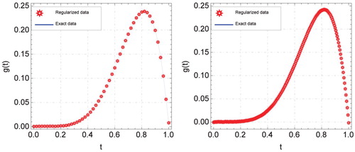
Figure 4. Graphs of exact and regularized data functions for $g(t)$ using new discrete mollification with $\epsilon =0.01$, N = 50 (left panel), and with $\epsilon =0.01$, N = 200 (right panel) for Example 1.

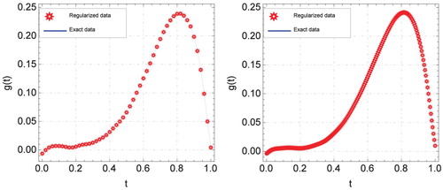
Figure 5. Graphs of noisy data function $g(t)$ (left panel) and exact and regularized data functions (right panel) using new discrete mollification with $\epsilon =0.1$, N = 128 for Example 2.

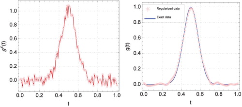
Figure 6. Graphs of exact and computed solutions for $q(t)$ with $\epsilon =1\mathrm{\%}$, $M_0=200$, N = 200 (left panel) and absolute error for $q(t)$ with $\epsilon =1\mathrm{\%}$, $M_0=200$, N = 200 (right panel) for Example 3.

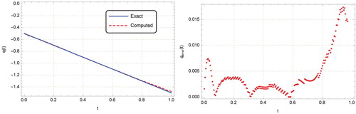
Figure 7. Graphs of exact and computed solutions for $q(t)$ with $\epsilon =5\mathrm{\%}$, $M_0=200$, N = 200 (left panel) and absolute error for $q(t)$ with $\epsilon =0.05$, $M_0=200$, N = 200 (right panel) for Example 3.

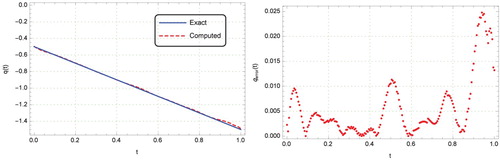
Figure 8. Graphs of exact and computed solutions for $p(t)$ with $\epsilon =1\mathrm{\%}$, $M_0=300$, N = 300 (left panel) and absolute error for $p(t)$ with $\epsilon =1\mathrm{\%}$, $M_0=350$, N = 350 (right panel) for Example 3.

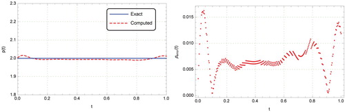
Figure 9. Graphs of exact and computed solutions for $p(t)$ with $\epsilon =5\mathrm{\%}$, $M_0=300$, N = 300 (left panel) and absolute error for $p(t)$ with $\epsilon =5\mathrm{\%}$, $M_0=350$, N = 350 (right panel) for Example 3.

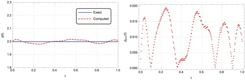
Figure 10. Graph of absolute error for $u(x,t)$ with $\epsilon =5\mathrm{\%}$, $M_0=250$, N = 250 for Example 3.

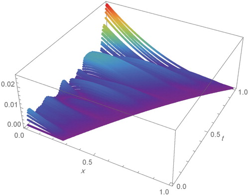
Table 3. RMS and $L_{\mathrm{\infty }}$ for Example 3.

ϵ	$M_0$	N	RMS for $q(t)$	RMS for $p(t)$	$L_{\mathrm{\infty }}$ for $u(x,t)$
$1\mathrm{\%}$	100	100	0.0141423	0.02565570	0.0293676
$5\mathrm{\%}$	100	100	0.0162337	0.02684790	0.0545190
$1\mathrm{\%}$	400	400	0.0058772	0.00824457	0.0117544
$5\mathrm{\%}$	400	400	0.0061947	0.01092980	0.0144669

Figure 11. Graphs of exact and computed solutions for $q(t)$ with $\epsilon =1\mathrm{\%}$, $M_0=200$, N = 200 (left panel) and absolute error for $q(t)$ with $\epsilon =1\mathrm{\%}$, $M_0=200$, N = 200 (right panel) for Example 4.

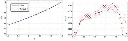
Figure 12. Graphs of exact and computed solutions for $q(t)$ with $\epsilon =5\mathrm{\%}$, $M_0=200$, N = 200 (left panel) and absolute error for $q(t)$ with $\epsilon =5\mathrm{\%}$, $M_0=200$, N = 200 (right panel) for Example 4.

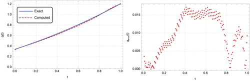
Figure 13. Graphs of exact and computed solutions for $p(t)$ with $\epsilon =1\mathrm{\%}$, $M_0=200$, N = 200 (left panel) and absolute error for $p(t)$ with $\epsilon =1\mathrm{\%}$, $M_0=200$, N = 200 (right panel) for Example 4.

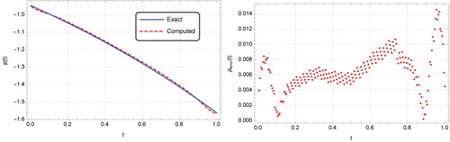
Figure 14. Graphs of exact and computed solutions for $p(t)$ with $\epsilon =5\mathrm{\%}$, $M_0=200$, N = 200 (left panel) and absolute error for $p(t)$ with $\epsilon =5\mathrm{\%}$, $M_0=200$, N = 200 (right panel) for Example 4.

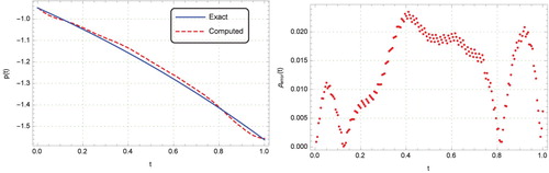
Figure 15. Graph of absolute error for $u(x,t)$ with $\epsilon =5\mathrm{\%}$, $M_0=250$, N = 250 for Example 4.

Table 4. RMS and $L_{\mathrm{\infty }}$ for Example 4.

ϵ	$M_0$	N	RMS for $q(t)$	RMS for $p(t)$	$L_{\mathrm{\infty }}$ for $u(x,t)$
$1\mathrm{\%}$	100	100	0.0150765	0.0155459	0.029597
$5\mathrm{\%}$	100	100	0.0160329	0.0176684	0.0303233
$1\mathrm{\%}$	400	400	0.00560614	0.0079557	0.0107032
$5\mathrm{\%}$	400	400	0.0061947	0.0100549	0.0145528

Murio DA. Mollification and space marching, In: Woodbury, K ed. Inverse Engineering Handbook, CRC Press;2002.

 Google Scholar