The bi-Helmholtz equation with Cauchy conditions: ill-posedness and regularization methods

Figures & data

Figure 1. Left: Exact solution of problem (3(3) $\begin{array}{rl}& \frac{{\mathrm{\partial }}^{4}u}{\mathrm{\partial }{x}^4}+2\frac{{\mathrm{\partial }}^{4}u}{\mathrm{\partial }{x}^2\mathrm{\partial }{y}^2}+\frac{{\mathrm{\partial }}^{4}u}{\mathrm{\partial }{y}^4}-2\frac{{\mathrm{\partial }}^{2}u}{\mathrm{\partial }{x}^2}-2\frac{{\mathrm{\partial }}^{2}u}{\mathrm{\partial }{y}^2}+u=0,(x,y)\in (0,1)\times \mathbb{R},\\ & \frac{{\mathrm{\partial }}^{j}u(0,y)}{\mathrm{\partial }{x}^j}={\phi }_j\left(y\right),j=1,2,3,4,y\in \mathbb{R}.\end{array}$(3) ) for ${\phi }_1\left(y\right)=e^{-y^2},{\phi }_i\left(y\right)=0,i=2,3,4.$ Right: The corresponding error of unregularized solution (7(7) $\begin{array}{rl}u(x,y;ϵ)& =u(x,y)+\frac{1}{2}ϵ\sin \left(\frac{y}{ϵ}\right)\\ & \times \left(2\cosh \left(x\sqrt{\frac{1}{{ϵ}^2}+1}\right)-x\sqrt{\frac{1}{{ϵ}^2}+1}\sinh \left(x\sqrt{\frac{1}{{ϵ}^2}+1}\right)\right).\end{array}$(7) ), with $ϵ=\frac{1}{10}$.

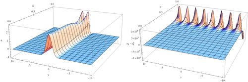
Table 1. The corresponding errors of wavelet regularized solution $u^{ϵ,W}$ of problem (19(19) $\begin{array}{r}\left\{\begin{array}{ll}{\mathrm{\Delta }}^{2}u-2\mathrm{\Delta }u+u=0,& \mathrm{i}\mathrm{n}(0,1)\times \mathbb{R},\\ u(0,y)={\mathrm{e}}^{-y^2}\cos 3y,& y\in \mathbb{R},\\ \frac{{\mathrm{\partial }}^{j}u(0,y)}{\mathrm{\partial }{x}^j}=0,j=1,2,3,& y\in \mathbb{R},\end{array}\right.\end{array}$(19) ) for various values of $x$ and $ϵ$.

$x$	$ϵ$	$\delta$	$\hat{J}$	$\parallel u-u^{ϵ,W}{\parallel }_2$
$x$thinsp;= 0.5	1E−1	2.0480E−2	4	2.6495E−2
	1E−5	1.6908E−6	4	1.0492E−2
	1E−15	1.7408E−16	5	5.6018E−4
$x$ = 0.7	1E−1	1.4270E−2	4	3.7860E−2
	1E−5	1.5322E−6	4	3.3792E−2
	1E−15	1.7580E−16	5	6.7418E−3
$x$ = 0.9	1E−1	1.8868E−2	4	3.1046E−1
	1E−5	1.9293E−6	4	2.1362E−1
	1E−15	1.8336E−16	5	4.8179E−2

Table 2. The corresponding errors of wavelet regularized solution $u^{ϵ,W}$ of problem (20(20) $\begin{array}{r}\left\{\begin{array}{ll}{\mathrm{\Delta }}^{2}u-2\mathrm{\Delta }u+u=0,& \mathrm{i}\mathrm{n}(0,1)\times \mathbb{R},\\ u(0,y)=0,& y\in \mathbb{R},\\ \frac{\mathrm{\partial }u(0,y)}{\mathrm{\partial }x}={\mathrm{e}}^{-y^2}\cos 3y,& y\in \mathbb{R},\\ \frac{{\mathrm{\partial }}^{j}u(0,y)}{\mathrm{\partial }{x}^j}=0,j=2,3,& y\in \mathbb{R}.\end{array}\right.\end{array}$(20) ) for various values of $x$ and $ϵ$.

x	ε	δ	$\hat{J}$	$\parallel u-u^{ϵ,W}{\parallel }_2$
x = 0.5	1E−1	1.6078E−2	4	1.8078E−2
	1E−5	1.9993E−6	4	6.0924E−3
	1E−15	1.4811E−16	5	1.7472E−4
x = 0.7	1E−1	1.57497E−2	4	2.4284E−2
	1E−5	1.7295E−6	4	7.5344E−3
	1E−15	1.6946E−16	5	4.4322E−4
x = 0.9	1E−1	1.3650E−2	4	4.3072E−1
	1E−5	1.9062E−6	4	2.1852E−2
	1E−15	1.5772E−16	5	4.6769E−3

Figure 2. Case 1 of Example 5.2. Plots of the wavelet regularized solutions for $ϵ=0.05,0.0005$ at left and middle, respectively. Right: plot of absolute errors versus $1/ϵ$ at $x$ = 0.8.

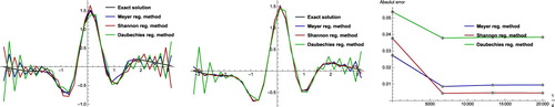
Figure 3. Case 2 of Example 5.2. Plots of wavelet regularized solutions for $ϵ=0.05,0.0005$ at left and middle, respectively. Right: plot of absolute errors versus $1/ϵ$ at $x$ = 0.8.

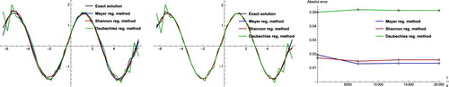
Figure 4. First row: plots of threshold regularized solutions for Example 5.3 at $x$ = 0.5 for $ϵ={10}^{-5},{10}^{-10},{10}^{-15}$ from left to right, respectively, with $N$ = 32. Second row: plots of the corresponding wavelet regularized solutions of first row by using Shannon wavelet.

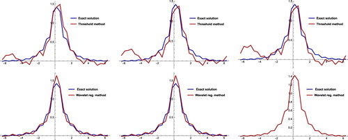
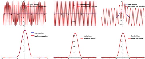
Figure 5. First row: plots of exact solutions of problem (23(23) $\begin{array}{rl}& {\mathrm{\Delta }}^{2}u-2\mathrm{\Delta }u+u=0,\mathrm{i}\mathrm{n}(0,1)\times \mathbb{R},\\ & u(0,y)={\mathrm{e}}^{-y^2},y\in \mathbb{R},\\ & \frac{{\mathrm{\partial }}^{j}u(0,y)}{\mathrm{\partial }{x}^j}=0,j=1,2,3,y\in \mathbb{R},\end{array}$(23) ) in Example 5.4 with / without noisy data at $x$ = 0.8 for $ϵ=0.05,0.005,0.0005,$ from left to right, respectively, where $N$ = 128. Second row: plots of exact and Fourier regularized solutions of problem(23(23) $\begin{array}{rl}& {\mathrm{\Delta }}^{2}u-2\mathrm{\Delta }u+u=0,\mathrm{i}\mathrm{n}(0,1)\times \mathbb{R},\\ & u(0,y)={\mathrm{e}}^{-y^2},y\in \mathbb{R},\\ & \frac{{\mathrm{\partial }}^{j}u(0,y)}{\mathrm{\partial }{x}^j}=0,j=1,2,3,y\in \mathbb{R},\end{array}$(23) ) in Example 5.4 with $\mathcal{N}=9,13,18$ at $x$ = 0.8 from left to right, respectively.

Table 3. The corresponding errors of Fourier regularized solution $u^{ϵ,F}$ of problem (23(23) $\begin{array}{rl}& {\mathrm{\Delta }}^{2}u-2\mathrm{\Delta }u+u=0,\mathrm{i}\mathrm{n}(0,1)\times \mathbb{R},\\ & u(0,y)={\mathrm{e}}^{-y^2},y\in \mathbb{R},\\ & \frac{{\mathrm{\partial }}^{j}u(0,y)}{\mathrm{\partial }{x}^j}=0,j=1,2,3,y\in \mathbb{R},\end{array}$(23) ) in Example 5.4 for s = 1 and various values of x and ε.

x	ε	δ	$M_{max}$	$\parallel u-u^{ϵ,F}{\parallel }_2$
x = 0.5	5E−2	3.1250E−3	9	1.2903E−4
	5E−3	3.1250E−4	13	7.4511E−7
	5E−4	3.1250E−5	18	1.3292E−9
x = 0.7	5E−2	3.1250E−3	9	1.2480E−4
	5E−3	3.1250E−4	13	1.1524E−5
	5E−4	3.1250E−5	18	4.1378E−7
x = 0.9	5E−2	3.1250E−3	9	2.0536E−3
	5E−3	3.1250E−4	13	1.8255E−3
	5E−4	3.1250E−5	18	1.8241E−3