Figures & data
Table 1. Conductivity parameters used in numerical experiments.
Figure 1. Comparison of the traditional 'first reconstruct then segment' scheme with the proposed 'simultaneously reconstruct and segment' scheme. The results on the right hand side are both segmented images, of which only the one from the simultaneous approach is guaranteed to satisfy the physically obtained EM data.
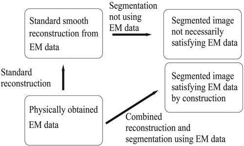
Figure 2. Opposing arrays of sources and receivers with shielded cage in between. The interior of the box is hidden behind the shields. The sources and receivers are only located on top and bottom of the box, but other setups are also possible. Left: Complete set up of imaging the contents of a shielded cage. Right: Schematic of shielding in z direction. The domain of interest is between these shields in each direction.
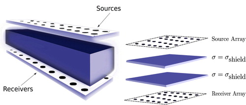
Figure 3. 2D Visualization of level set representation described in (Equation10(10)
(10) ); In this schematic visualization, it is assumed that the individual regions
and
are both disc-shaped, but that the specific rule (Equation10
(10)
(10) ) specifies which value to take in the overlap region
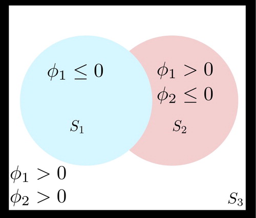
Table 2. Conductivity parameters used in numerical experiments.
Figure 4. Surface plots of 3D shape evolution for Numerical Experiment 1. Shown are the initial shape and snapshots at iteration numbers and the true phantom. The surrounding shields are not shown here. In the online version of this paper, the colour red indicates the shape of the conductivity
and blue indicates the shape of the conductivity
. The third region is transparent and represents air (
).
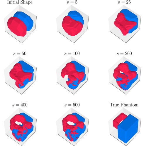
Figure 5. Line search analysis of LK-colour level set reconstruction for Numerical Experiment 1. Top row: Evolution of the average number of voxels as a function of the sweep number s. The dotted (and yellow in the online version of the paper) line represents
and the solid (black in the online version) line represents
. Middle row: Evolution of the step sizes
and
, denoted in the online version by yellow and black lines. Bottom row: Evolution of pseudo-cost
as a function of the sweep number s.
![Figure 5. Line search analysis of LK-colour level set reconstruction for Numerical Experiment 1. Top row: Evolution of the average number of voxels N¯ as a function of the sweep number s. The dotted (and yellow in the online version of the paper) line represents N¯s1 and the solid (black in the online version) line represents N¯s2. Middle row: Evolution of the step sizes τ1s and τ2s , denoted in the online version by yellow and black lines. Bottom row: Evolution of pseudo-cost J~[Φ]s as a function of the sweep number s.](/cms/asset/1b8f1a73-cd4c-4bb9-9996-e074e81cd1de/gipe_a_1797003_f0005_oc.jpg)
Figure 6. 2D cross-sections through a 3D reconstruction for Numerical Experiment 1 using different regularization schemes. Shown is the container region including shields. Each row: Left z = 25, middle , right y = 18. 1st row: LK-Pixel, 2nd row: LK-single-level set
, 3rd row: LK-single-level set
, 4th row: LK-colour level set and 5th row: true phantom.
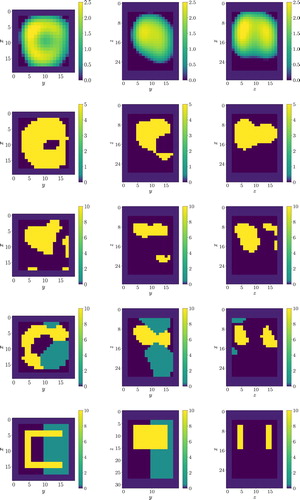
Figure 7. Pseudo-cost for four different regularization schemes; LK-colour level set, LK-single-level set, LK-pixel and SD-pixel.
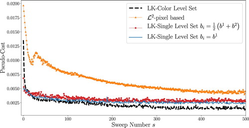
Figure 8. Left: Sample of conductivity profile in using probability distribution
, Middle: Sample of conductivity profile in
using probability distribution
, Right: Sample of conductivity profile in
using probability distribution
.
Figure 9. 2D cross-sections through a 3D reconstruction for Numerical Experiment 1 using the formulation in (Equation22(22)
(22) ) for the true phantom. Here,
is drawn from a normal distribution with parameters
. Each row: Left z = 23, middle x = 15, right y = 18 Top: true phantom, Bottom: LK-colour level set reconstruction at sweep s = 1000.
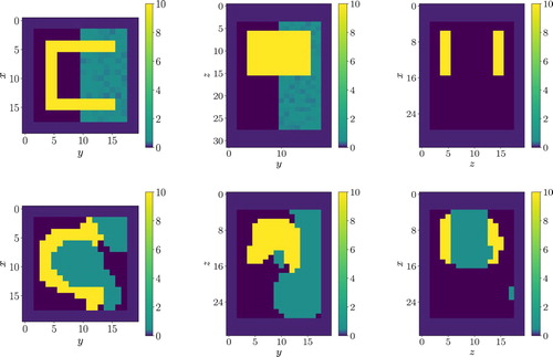
Figure 10. 2D cross-sections through a 3D reconstruction for Numerical Experiment 1 using the formulation in (Equation22(22)
(22) ) for the true phantom. Here,
is drawn from a uniform distribution with parameter
. Each row: Left z = 23, middle x = 15, right
Top: True Phantom, Bottom: LK-colour level set reconstruction at sweep s = 10000
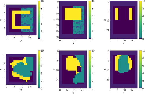
Figure 11. 2D cross-sections through a 3D reconstruction for Numerical Experiment 1 using the formulation in (Equation22(22)
(22) ) for the true phantom. Here,
is drawn from a normal distribution with parameters
. Each row: Left z = 23, middle x = 15, right y = 18 Top: true phantom, Bottom: LK-colour level set reconstruction at sweep s = 1000.
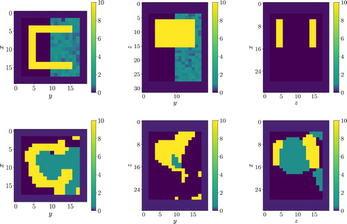
Figure 12. Pseudo-cost comparison between different sampling methods for creating conductivity profile associated with .
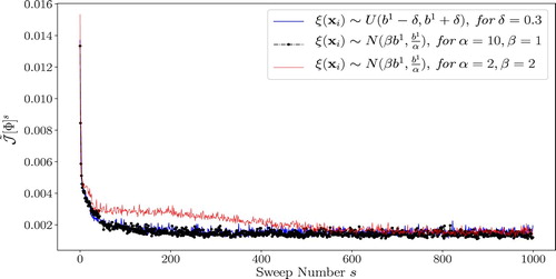
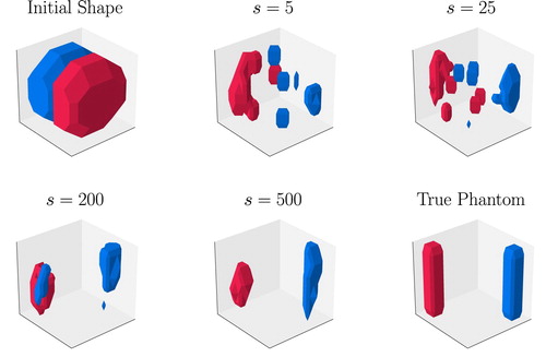
Figure 13. Surface plots of 3D shape evolution for Numerical Experiment 2. Shown are the initial shape and snapshots at iteration numbers and the true phantom. The surrounding shields are not shown here. In the online version of this paper, the colour red indicates the shape of the conductivity
and blue indicates the shape of the conductivity
.
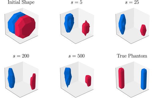
Figure 14. Surface plots of 3D shape evolution for Numerical Experiment 2 with an initial seeding phase where . The surrounding shields are not shown here. Displayed are the initial shape and snapshots at iteration numbers s = 5, 25, 200, 500 and the true phantom. In the online version of this paper, the colour red indicates the shape of the conductivity
and blue indicates the shape of the conductivity
.