Figures & data
Figure 1. The experimental site.
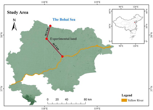
Figure 2. The distribution map of multi-year rainfall and temperature.
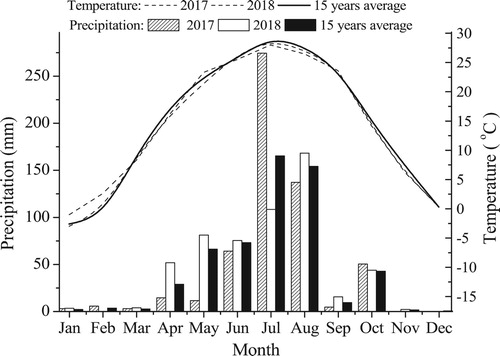
Figure 3. The structure and planting map of raised fields. (A) sectional drawing of a raised field (blue arrow represents summer precipitation, and red arrow represents winter groundwater), (B) vertical view (red asterisk represent sampling plots in the central regions, black asterisk represent sampling plots in the marginal regions, and number of asterisks represent the sampling numbers), (C) the intercropping of winter wheat or summer maize with forestry in the central regions, (D) either winter wheat or summer maize were planted alternately in the central regions.
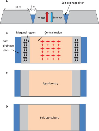
Figure 4. The variations in soil electrical conductivity at depths of 0–30 cm in normal fields and raised fields. The soil electrical conductivity is the average value from the central and marginal regions of soil. The average values, e.g. 3.0 and 4.0 mS/cm 25°C, respectively, represent 3.6 and 5 ‰ NaCl contents in soil at depths of 0–30 cm (soil tillage layer).
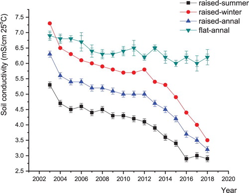
Table 1. Water sources of crop leaves and crop intrinsic water use efficiency (iWUE) during winter wheat seasons in the central regions and marginal regions under single agriculture in raised fields (SAR) mode (mean ± standard deviation in brackets).
Table 2. Water sources of crop leaves and crop intrinsic water use efficiency (iWUE) during summer maize seasons in the central regions and marginal regions under single agriculture in raised fields (SAR) mode (mean ± standard deviation in brackets).
Table 3. Water sources of topsoil and soil electrical conductivity of the saturation extract (ECse) during winter wheat seasons in the central regions and marginal regions under single agriculture in raised fields (SAR) mode (mean ± standard deviation in brackets).
Table 4. Water sources of topsoil and soil electrical conductivity of the saturation extract (ECse) during summer maize seasons in the central regions and marginal regions under single agriculture in raised fields (SAR) mode (mean ± standard deviation in brackets).
FIgure 5. The biomass yield of crops in the central regions from 2015 to 2018. SAR: single agriculture in raised fields, FAR: agroforest in raised fields, Biomass yield: the sum of the grains and stalks of winter wheat or summer maize.
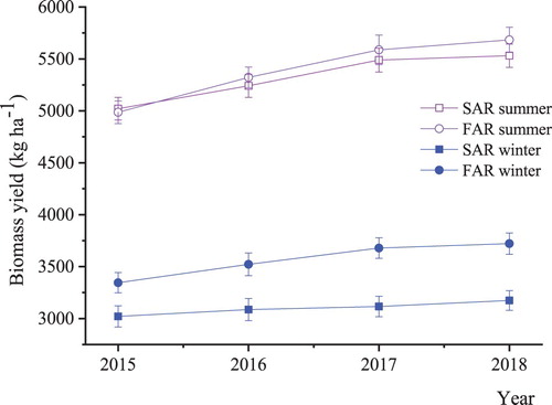
Table 5. Water sources of crop leaves and crop intrinsic water use efficiency (iWUE) during winter wheat seasons under the single agriculture in raised fields (SAR) and agroforest in raised fields (FAR) modes (mean ± standard deviation in brackets).
Table 6. Water sources of topsoil and soil electrical conductivity of the saturation extract (ECse) during winter wheat seasons under the single agriculture in raised fields (SAR) and agroforest in raised fields (FAR) modes (mean ± standard deviation in brackets).
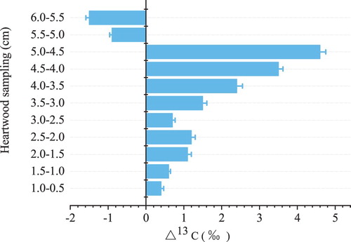
Figure 6. The distribution of δ13C (‰) values in the heartwood of trees under agroforest in raised fields. The wood cores were sliced at intervals of 0.5 cm without bark from the bark side to the heartwood. For example, 1–0.5 cm represents using the ‘previous’ δ13C value minus the ‘current’ δ13C value. If the δ13C difference value is positive (+), it means that the ‘previous’ δ13C value greater than that of the ‘current.’ If the δ13C difference value is negative (−), it means that the ‘previous’ δ13C value less than that of the ‘current.’