Figures & data
Figure 1. Illustration of (a) racing motorcycle front fairing as well as (b) considered segment in back view showing the socket for mounting on the vehicle and the ribbed reinforcement substructure with exemplary indication of wall thicknesses.
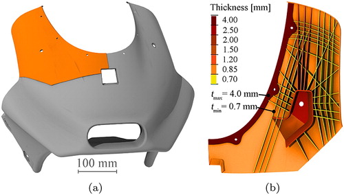
Figure 2. Volume element with principal material directions indicated via ∥- and ⊥-symbols.
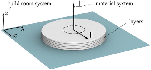
Figure 3. Rendering of (a) coupon orientations (Sindinger et al. Citation2020) with ϕ indicating the inclination angle to the build layer plane (xy) and consequently the loading direction (red arrows) as well as (b) component build layout.
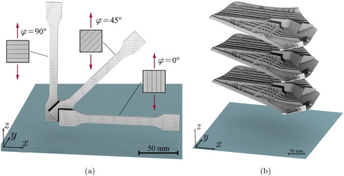
Table 1. Laser parameters.
Figure 4. Depiction of (a) fixture with sample glued onto a machined aluminium block that is screwed onto a swivel mount and loaded via indenter probe. (b) Entire setup with servo-hydraulic actuator, DIC cameras and spotlight. (c) Inclinometer for recording the swivel mount orientation.
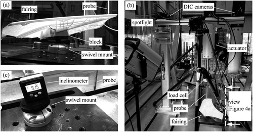
Figure 5. FE model with 2 mm mesh size, constrained nodes at block contact in green and detail enforced displacement direction indicated by red arrow with corresponding multi-point constraints in blue.
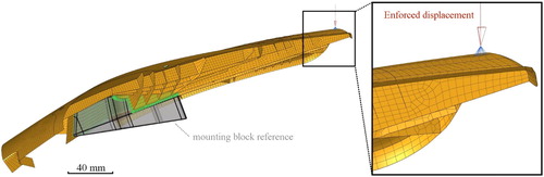
Figure 6. Mesh convergence with normalised deviation of reaction force for 1.5 mm displacement at load location on the left and number of elements (N) on the right axis with chosen size (dotted line).
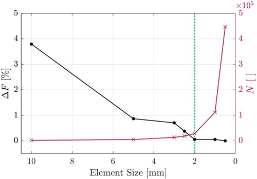
Figure 7. Schematic of shell element with nodes N1-4, local 1,2,3-, global x,y,z- and axisymmetric material -coordinate system as well as out-of-plane angles ϕ for the respective element directions.
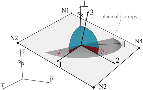
Table 2. Coefficient of determination  .
.
Figure 8. (a) 3D scan-based contour plot showing deviation d of the produced part to the CAD model in z-direction with cutting plane indicated via dashed lines and (b) cut view of overlayed CAD (black) and scan reconstruction (orange).
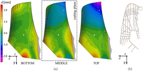
Figure 9. Visualisation of the curve fitting result (top) and the full material model approximating the dependency on orientation in the polar domain from 0 to 90 and thickness (bottom), with markers indicating tensile test data and coloured lines the fitted functions for (a) Young's modulus and (b) Poisson's ratio.
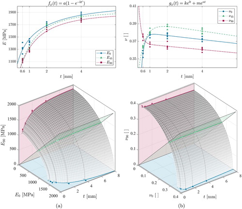
Figure 10. (a) Reaction force–displacement curves of the averaged physical test in blue (SD indicated by shaded region) and the different FE simulation results for homogeneous and mapped material properties. Markers show onset of buckling during the test at D = 2.6 mm and the maximum displacement (D = 5.0 mm), with corresponding extracted video stills (blue frame). For comparison, also the buckled shell element mesh is shown (red frame). (b) Error in percent with respect to the experimental mean value for the marker locations.
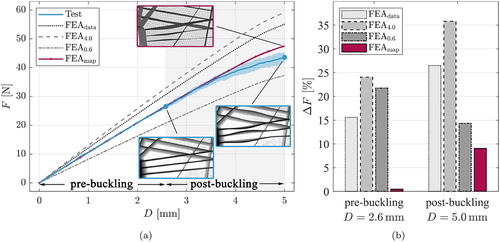
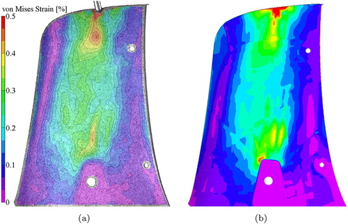
Figure 11. Von Mises strain at displacement D = 5 mm for (a) DIC data obtained during experiments and (b) FE simulation considering anisotropic thickness dependency of material properties.