
Figures & data
Figure 1. Additive manufacturing processes for metals and their basic features.
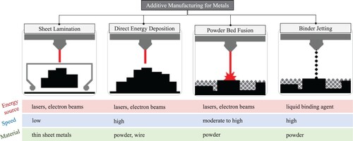
Figure 2. Schematic representation of a PBF and a co-axial DED process. Courtesy of Dr. Florian Wirth for the experimental images taken at the Institute of Machine Tools & Manufacturing at ETH Zurich [Citation26].
![Figure 2. Schematic representation of a PBF and a co-axial DED process. Courtesy of Dr. Florian Wirth for the experimental images taken at the Institute of Machine Tools & Manufacturing at ETH Zurich [Citation26].](/cms/asset/e936184b-b950-4ebb-adb5-8ad21b7b0858/nvpp_a_2274494_f0002_oc.jpg)
Figure 3. Different scales of study in modelling MAM processes (top) and the fundamental physical phenomena occurring in and around the melt pool region at the scale of the powder (bottom).
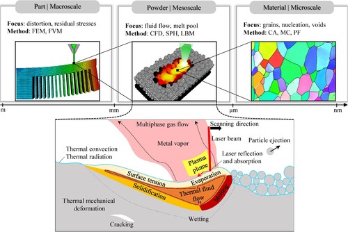
Figure 4. Schematic of Young's relation: simplification to planar geometry in wetting surfaces.
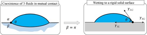
Figure 5. Discrete powder models in MAM: (A) Spherical powder model using DEM adapted from Chen et al. [Citation54]; (B) non-spherical powder models represented by multi-spheres and super-ellipsoids adapted from [Citation55].
![Figure 5. Discrete powder models in MAM: (A) Spherical powder model using DEM adapted from Chen et al. [Citation54]; (B) non-spherical powder models represented by multi-spheres and super-ellipsoids adapted from [Citation55].](/cms/asset/96eafecb-9d19-4317-9dd2-98a5a3bf3949/nvpp_a_2274494_f0005_oc.jpg)
Figure 6. Ishikawa diagram representing key parameters affecting the metal powder quality in AM.
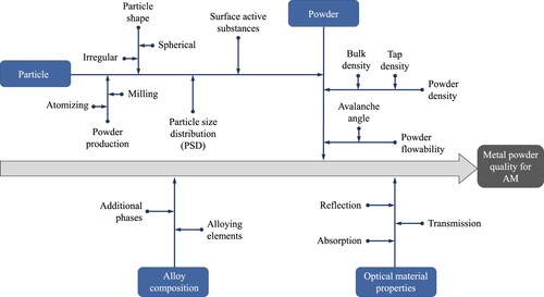
Figure 7. A close-up of the laser-powder interaction in PBF for two selected particles (A) and the temperature isosurface of the two particles (B), taken from [Citation63].
![Figure 7. A close-up of the laser-powder interaction in PBF for two selected particles (A) and the temperature isosurface of the two particles (B), taken from [Citation63].](/cms/asset/71b9a23e-7c4a-4307-92b2-0f2d3b2cd297/nvpp_a_2274494_f0007_oc.jpg)
Figure 8. Two heat source modelling approaches widely used in simulating MAM processes: volumetric and ray tracing.
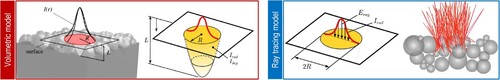
Figure 9. Perceptual analogy between subtractive and additive manufacturing: Similarity of the critical regions (blue frames) and viewing the melt pool as a non-physical tool in AM.
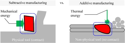
Table 1. Summary of publications from the leading research groups in MAM simulations with hardware-accelerated particle methods.
Figure 10. A general classification of numerical techniques, highlighting the category of particle-based methods.
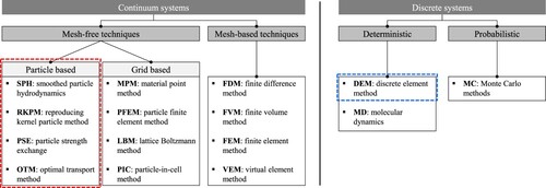
Figure 11. Illustration of the contact interactions between two DEM particles and the diagram of resultant forces acting on particle j.
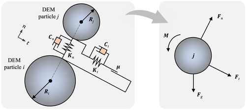
Figure 12. Illustration of the SPH approximation scheme in 2D. Spatial discretization by material points or particles (red circles) is shown at the initial () and current (
) configurations. Support domain of material point or particle i and its affected neighbours (i.e. green circles) are updated at each time step.
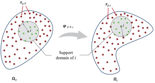
Figure 13. Initial triangulation of the domain and illustration of the OTM approximation scheme in 2D. Spatial discretization by nodal points (white squares) and material points (red circles) is shown at the initial () and current (
) configurations. Support domain of material point i and its affected nodes (i.e. green squares) are updated at each time step.
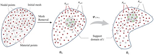
Figure 14. Screenshots of a powder recoating model using DEM (left) and particle size distribution with its colour code definition (right), reprinted from Meier et al. [Citation110] with permission from Elsevier.
![Figure 14. Screenshots of a powder recoating model using DEM (left) and particle size distribution with its colour code definition (right), reprinted from Meier et al. [Citation110] with permission from Elsevier.](/cms/asset/569fb749-6b22-41c7-a56b-a17198e6590a/nvpp_a_2274494_f0014_oc.jpg)
Figure 15. Coupled DEM-CFD modelling framework of powder packing and melt pool simulation in a multi-layer electron beam melting process by Yan et al. [Citation125], reprinted with permission from Elsevier.
![Figure 15. Coupled DEM-CFD modelling framework of powder packing and melt pool simulation in a multi-layer electron beam melting process by Yan et al. [Citation125], reprinted with permission from Elsevier.](/cms/asset/92db4a9b-5183-4b2d-8930-1b18a0f71fac/nvpp_a_2274494_f0015_oc.jpg)
Table 2. Summary of notable DEM-based powder spreadability analyses in MAM (since 2018).
Figure 16. 2D mesoscopic SPH simulations of PBF. (A) Russell et al. [Citation42] using a robust weakly-compressible SPH for simulating a PBF process at the powder scale, spending ≈ 36 hours for simulating a 1-mm long track; (B) The distributions of the velocity field temperature in a single-layer PBF track performed by Liu et al. [Citation131]; (C) The first multi-resolution SPH simulation of a PBF process, running 2x faster than a single-resolution model, developed by Afrasiabi et al. [Citation132]. The state scale is linear, starting from the liquid state represented by red, down to the solid state shown in blue.; (D) Multi-layer PBF simulation enabled by integrating a rainfall-like rigid powder model into the SPH thermal-fluid solver, presented in [Citation133].
![Figure 16. 2D mesoscopic SPH simulations of PBF. (A) Russell et al. [Citation42] using a robust weakly-compressible SPH for simulating a PBF process at the powder scale, spending ≈ 36 hours for simulating a 1-mm long track; (B) The distributions of the velocity field temperature in a single-layer PBF track performed by Liu et al. [Citation131]; (C) The first multi-resolution SPH simulation of a PBF process, running 2x faster than a single-resolution model, developed by Afrasiabi et al. [Citation132]. The state scale is linear, starting from the liquid state represented by red, down to the solid state shown in blue.; (D) Multi-layer PBF simulation enabled by integrating a rainfall-like rigid powder model into the SPH thermal-fluid solver, presented in [Citation133].](/cms/asset/1ff81002-7c6f-49da-8ca6-747f90cf0327/nvpp_a_2274494_f0016_oc.jpg)
Figure 17. 3D SPH simulations of PBF: (A) Fürstenau et al. [Citation92]; (B) Weirather et al. [Citation36]; (C) Liu et al. [Citation134]; (D) Qiu et al. [Citation135]; (E) Meier et al. [Citation96, Citation136]; (F) Dao and Lou [Citation94]. Images are adapted from the original publications with permission.
![Figure 17. 3D SPH simulations of PBF: (A) Fürstenau et al. [Citation92]; (B) Weirather et al. [Citation36]; (C) Liu et al. [Citation134]; (D) Qiu et al. [Citation135]; (E) Meier et al. [Citation96, Citation136]; (F) Dao and Lou [Citation94]. Images are adapted from the original publications with permission.](/cms/asset/e3c5c9f1-bbb4-428d-b88b-98425164f295/nvpp_a_2274494_f0017_oc.jpg)
Figure 18. 3D high-fidelity simulation with single- and multi-resolution SPH. (A) High-fidelity PBF simulation with a single-resolution SPH scheme to quantify the effects of recoil pressure and Marangoni forces on the melt pool geometry, taken from Afrasiabi et al. [Citation139]; (B) Four solidified parallel tracks and surface height values in a multi-track PBF process simulated by the multi-resolution SPH code of Lüthi et al. [Citation140]. The discretization size varies from 61.8 (coarsest) to 3.8 (finest) μm.
![Figure 18. 3D high-fidelity simulation with single- and multi-resolution SPH. (A) High-fidelity PBF simulation with a single-resolution SPH scheme to quantify the effects of recoil pressure and Marangoni forces on the melt pool geometry, taken from Afrasiabi et al. [Citation139]; (B) Four solidified parallel tracks and surface height values in a multi-track PBF process simulated by the multi-resolution SPH code of Lüthi et al. [Citation140]. The discretization size varies from 61.8 (coarsest) to 3.8 (finest) μm.](/cms/asset/a981d52d-4317-4959-b700-04700e09e08e/nvpp_a_2274494_f0018_oc.jpg)
Figure 19. Overview of fusion-based MAM simulation using OTM schemes. (A) A 7 mm PBF track simulated by Fan and Li [Citation141] using adaptive (mesh) discretization size ranging from 25–1000 μm in an HOTM setup; (B) Fan et al. [Citation93] using the same method but at a much higher resolution using about 1.3 million material points for a 1.6 mm track; (C) Work of Wessels et al. [Citation46] on modelling the fusion of two metal particles fusion with a stabilised OTM code; (D) A similar metal particle fusion example simulated by Wessels et al. [Citation142] with an enhanced ray-tracing heat source model.
![Figure 19. Overview of fusion-based MAM simulation using OTM schemes. (A) A 7 mm PBF track simulated by Fan and Li [Citation141] using adaptive (mesh) discretization size ranging from 25–1000 μm in an HOTM setup; (B) Fan et al. [Citation93] using the same method but at a much higher resolution using about 1.3 million material points for a 1.6 mm track; (C) Work of Wessels et al. [Citation46] on modelling the fusion of two metal particles fusion with a stabilised OTM code; (D) A similar metal particle fusion example simulated by Wessels et al. [Citation142] with an enhanced ray-tracing heat source model.](/cms/asset/48a9c0be-4ee7-48dc-97fb-7294172edf68/nvpp_a_2274494_f0019_oc.jpg)
Figure 20. State of the art in particle-based simulation of DED. (A) Dao and Lou [Citation94] using approximately 1.2 million SPH particles in their initial attempt and spending about 7h on 24 supercomputer CPU cores for 0.5 ms of a DMD process; (B) Dao and Lou [Citation95] using 1.6 million SPH particles and spending about 230 h on 24-core parallel CPU nodes to simulate 0.5 s of the DED process in their more recent work; (C) work of Wang et al. [Citation107] using an in-house serial OTM code to simulate a single-track DED with depositing 200 metallic particles.
![Figure 20. State of the art in particle-based simulation of DED. (A) Dao and Lou [Citation94] using approximately 1.2 million SPH particles in their initial attempt and spending about 7h on 24 supercomputer CPU cores for 0.5 ms of a DMD process; (B) Dao and Lou [Citation95] using 1.6 million SPH particles and spending about 230 h on 24-core parallel CPU nodes to simulate 0.5 s of the DED process in their more recent work; (C) work of Wang et al. [Citation107] using an in-house serial OTM code to simulate a single-track DED with depositing 200 metallic particles.](/cms/asset/dc0bb9f1-6261-4c53-877f-243880074ead/nvpp_a_2274494_f0020_oc.jpg)
Figure 21. State of the art in multiphysics high-fidelity modelling of BJ with meshfree particle-based [Citation97] and mesh-based CFD [Citation147] simulation approaches.
![Figure 21. State of the art in multiphysics high-fidelity modelling of BJ with meshfree particle-based [Citation97] and mesh-based CFD [Citation147] simulation approaches.](/cms/asset/f5dd2d4d-73c4-4ea1-929c-42591c1a6e19/nvpp_a_2274494_f0021_oc.jpg)
Table 3. Overview of notable particle-based MAM simulations published in the past five years.
Figure 22. Comparative analysis of particle-based and mesh-based methods for multi-physics MAM process simulation at the powder scale, highlighting their respective capabilities and limitations. The utilisation of emojis serves to visually elucidate that the management of ‘Aspect X’ in MAM simulations is inherently more intuitive and efficient when employing particle-based or mesh-based techniques.
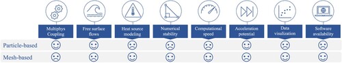
Figure 23. High-fidelity simulation of single-track laser PBF using: (left) DEM-SPH presented in [Citation97]; (right) DEM-CFD presented in [Citation158].
![Figure 23. High-fidelity simulation of single-track laser PBF using: (left) DEM-SPH presented in [Citation97]; (right) DEM-CFD presented in [Citation158].](/cms/asset/570e1540-a2fe-43d5-b54d-d37f50bb26fc/nvpp_a_2274494_f0023_oc.jpg)
Figure 24. Current state of the art in high-fidelity PBF simulation: the advanced DEM-CFD framework of Yu and Zhao [Citation163] accounting for nearly all physical effects, published in 2022. Images are adapted from the reference article with permission.
![Figure 24. Current state of the art in high-fidelity PBF simulation: the advanced DEM-CFD framework of Yu and Zhao [Citation163] accounting for nearly all physical effects, published in 2022. Images are adapted from the reference article with permission.](/cms/asset/ac249135-1619-4249-916f-d0d08bb33103/nvpp_a_2274494_f0024_oc.jpg)
Figure 25. Enhancing the current Beer-Lambert volumetric heat source model to a surface heat source modelling approach. Enhanced absorption model includes multiple laser-material interactions and provides more accurate results.
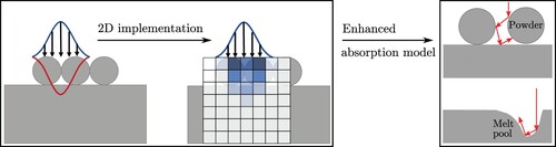
Figure 26. 3D-printed cube of 316L fabricated by more than 150 layers of PBF and several thousands of scan vectors.

Figure 27. Multi-track and multi-layer MAM simulations: (A) Buildup of 10 PBF layers simulated by a 2D SPH framework in [Citation133]; (B) A coupled DEM-SPH model of PBF for a few tracks of Ti-6Al-4V PBF [Citation164]; (C) Single-track multi-layer PBF simulation of [Citation165] using DEM-CFD; and (D) Multi-track multi-layer electron beam melting simulation of [Citation78, Citation125] using a multiphysics DEM-CFD framework.
![Figure 27. Multi-track and multi-layer MAM simulations: (A) Buildup of 10 PBF layers simulated by a 2D SPH framework in [Citation133]; (B) A coupled DEM-SPH model of PBF for a few tracks of Ti-6Al-4V PBF [Citation164]; (C) Single-track multi-layer PBF simulation of [Citation165] using DEM-CFD; and (D) Multi-track multi-layer electron beam melting simulation of [Citation78, Citation125] using a multiphysics DEM-CFD framework.](/cms/asset/499b1ddd-4882-4096-a0bc-8a2a3caa8086/nvpp_a_2274494_f0027_oc.jpg)
Figure 28. Recent multimaterial PBF models: (A) the 3D SPH framework of [Citation148] for a bi-metal powder system; (B) the 2D lattice-Boltzmann framework of [Citation171] for in-situ alloying of AB with two pure element powders A and B. Both works were published in 2021.
![Figure 28. Recent multimaterial PBF models: (A) the 3D SPH framework of [Citation148] for a bi-metal powder system; (B) the 2D lattice-Boltzmann framework of [Citation171] for in-situ alloying of AB with two pure element powders A and B. Both works were published in 2021.](/cms/asset/418bd518-5422-48b8-b104-a70a50fbd136/nvpp_a_2274494_f0028_oc.jpg)
Figure 29. 3D multimaterial PBF simulation using a combined DEM-SPH approach. The colour of DEM grains in the left image represents their diameter.
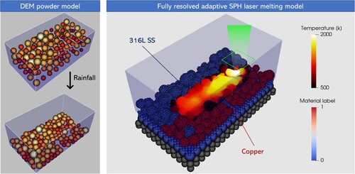
Figure 30. Promising applications of ML in metal additive manufacturing: (A) Prediction of melt pool dynamics and temperature using FEM and physics-informed neural networks (PINN) compared to experiment presented by Zhu et al. [Citation172]; (B) An efficient convolutional neural network architecture for fast melt pool temperature predictions in MAM that is about 5 orders of magnitude faster than Flow3D simulations, proposed by Hemmasian et al. [Citation173].
![Figure 30. Promising applications of ML in metal additive manufacturing: (A) Prediction of melt pool dynamics and temperature using FEM and physics-informed neural networks (PINN) compared to experiment presented by Zhu et al. [Citation172]; (B) An efficient convolutional neural network architecture for fast melt pool temperature predictions in MAM that is about 5 orders of magnitude faster than Flow3D simulations, proposed by Hemmasian et al. [Citation173].](/cms/asset/5150250f-8df8-4af5-8d80-90f0db4218df/nvpp_a_2274494_f0030_oc.jpg)