
Figures & data
Figure 1. The tropical island of Unguja (1700 km2, population 700,000, OCGS, Citation2010) is the largest of the Zanzibar Islands in Tanzania. The population is highly concentrated in the western urban area, while the rest of the island remains rural. The case study area is located in the south-central part of the island.
Figure 2. Individual land cover change trajectories (n = 81) were classified into six different qualitative change trajectory classes using a decision tree. These trajectories reflect stability, gain, loss, and turnover patterns of land cover changes. These trajectories were further scaled into degree of land cover quality following the idea that the more forested or scrub-covered landscape has been over the decades, the higher is the quality of the land cover.
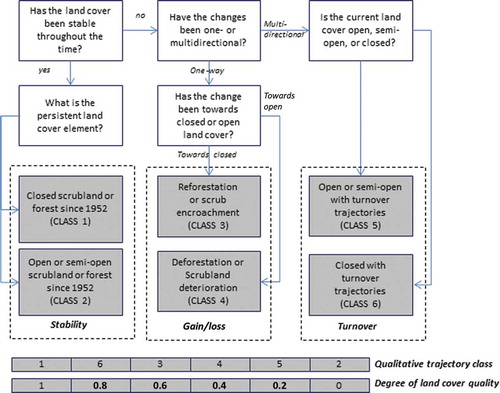
Figure 3. The process of creating generalised spatial data of land use patterns into four layers (a–d) based on the participatory mapping of 18 landscape services by local farmers.
Figure 4. Qualitative land cover change classes based on the change trajectory analysis show that the largest change classes are indicating either forest/scrubland (class 1) or open and semi-open land cover stability (class 2). Gains and losses of forest cover (classes 3 and 4) through reforestation and deforestation are typically small and spatially dispersed areas in the landscape. Around 20% of the land has changed between open and closed conditions with different turnover trajectories (classes 5 and 6). The figure represents also the boundary of the Jozani–Chwaka Bay National Park, covering the eastern part of the study area.
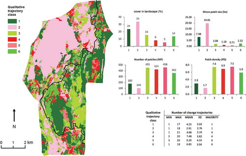
Figure 5. Two aggregated variables describing land cover changes at the spatial resolution of 200 m × 200 m cells (4 ha). The number of change trajectories (a) was calculated for each aggregated cell (hypothetical maximum 81). The degree of land cover quality (b) ranges from closed stable land cover areas (value 1) to open stable sites (value 0). Both figures represent also the boundary of the Jozani–Chwaka Bay National Park, covering the eastern part of the study area.
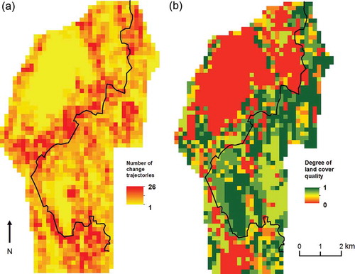
Figure 6. Community benefits as generalised land use patterns (200 m cell size): community-based dominant land use and resources (a), community-based non-material landscape benefits (b), intensity of all mapped landscape service points as Kernel density surface as points/ha (c), and richness of all mapped landscape service points (d). For layers a and b, figures in parentheses indicate the relative (%) spatial coverage. Each figure represents also the boundary of the Jozani–Chwaka Bay National Park, covering the eastern part of the study area.
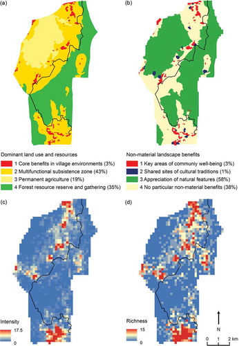
Figure 7. Spatial distribution of selected material and non-material landscape services mapped by 218 farmers during the participatory GIS campaign. Figures in parentheses indicate the absolute amount of mapped points. The boundary of the Jozani–Chwaka Bay National Park, covering the eastern part of the study area, is visualised on all maps.
Figure 8. Share (%) of different qualitative land cover change trajectories (1–6) within selected dominant land use (a) and non-material landscape benefit (b) classes and within the total land area (All).
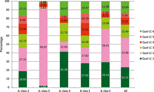
Figure 9. Mean and standard deviation of the degree of land cover quality (left) and number of change trajectories (right) in each dominant land use zone.
Table 1. Spatial relationship between the landscape change trajectory diversity, degree of land cover quality, distance from settlement, landscape service richness, and intensity calculated as Spearman’s rho correlation.