1,252
Views
6
CrossRef citations to date
0
Altmetric
Original Articles

Local sensitivity of per-recruit fishing mortality reference points

&
Pages 525-545 | Received 30 Dec 2015, Accepted 12 Aug 2016, Published online: 07 Sep 2016

Figures & data

Figure 1. Illustration of a precautionary approach fisheries harvest decision rule that involves stock status zones defined by RPs and a harvest rate limit RP. Fisheries may harvest less than the limit.
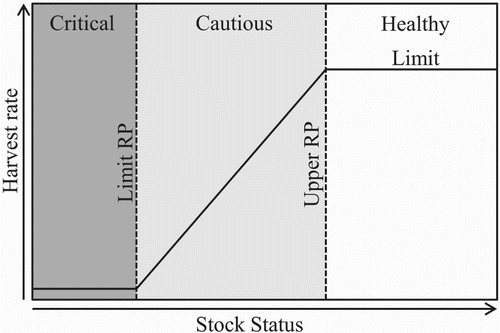
Figure 1. Illustration of a precautionary approach fisheries harvest decision rule that involves stock status zones defined by RPs and a harvest rate limit RP. Fisheries may harvest less than the limit.

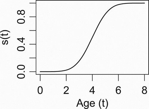
Figure 2. Selectivity function s(t) of age t for the illustrative example.

Figure 2. Selectivity function s(t) of age t for the illustrative example.

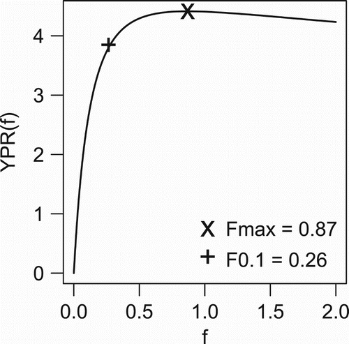
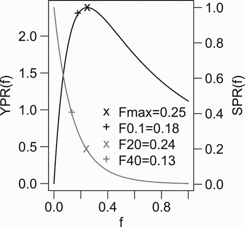
Figure 3. Illustration of a YPR curve and two fishing mortality RPs, Fmax and F0.1.

Figure 3. Illustration of a YPR curve and two fishing mortality RPs, Fmax and F0.1.

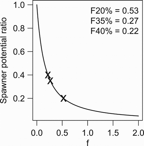
Figure 4. Illustration of a spawner potential ratio curve, SPR(f)/SPR(0), and three fishing mortality RPs, F20%,F35% and F40%.

Figure 4. Illustration of a spawner potential ratio curve, SPR(f)/SPR(0), and three fishing mortality RPs, F20%,F35% and F40%.

Figure 5. Solid black curves are values of F RPs for perturbed values of the Von Bertalanffy growth parameter k. Solid grey curves are the local slopes. Reference lines (grey dashed) indicate a local slope of zero and the corresponding value for k.
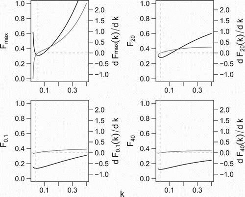
Figure 5. Solid black curves are values of F RPs for perturbed values of the Von Bertalanffy growth parameter k. Solid grey curves are the local slopes. Reference lines (grey dashed) indicate a local slope of zero and the corresponding value for k.

Figure 6. YPR divided by the maximum over f (scaled YPR) for different values of the VonB k parameter. The inset figure shows the maximum YPR (over f) versus k.
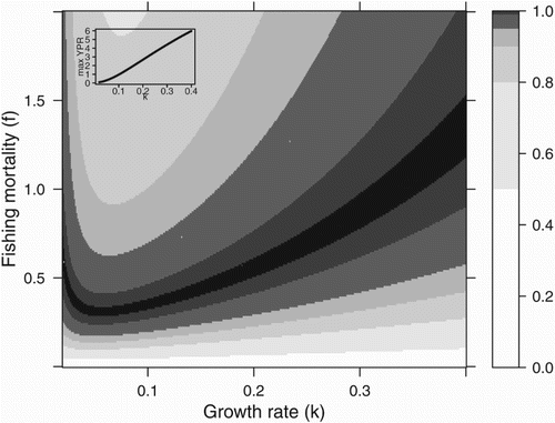
Figure 6. YPR divided by the maximum over f (scaled YPR) for different values of the VonB k parameter. The inset figure shows the maximum YPR (over f) versus k.

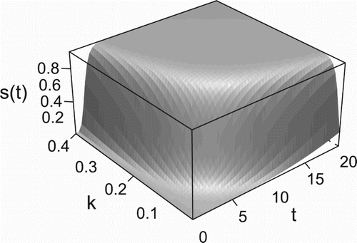
Figure 7. Selectivity function s(t) of age t that is a composite function of a selectivity function s~(l) of length l and a length function l(t) of age with growth rate parameter k. s(t)=s~{l(t)}.

Figure 7. Selectivity function s(t) of age t that is a composite function of a selectivity function s~(l) of length l and a length function l(t) of age with growth rate parameter k. s(t)=s~{l(t)}.

Figure 8. Solid black curves are values of F RPs for perturbed values of the Von Bertalanffy growth parameter k but a fixed k=0.2 in the length-based selectivity function. Dashed black curves are values of F RPs with perturbed k's in the selectivity function. Grey curves are F RPs scaled by the average selectivity at ages 0–20.
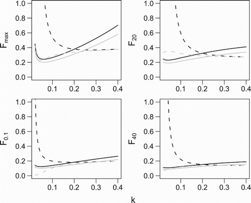
Figure 8. Solid black curves are values of F RPs for perturbed values of the Von Bertalanffy growth parameter k but a fixed k=0.2 in the length-based selectivity function. Dashed black curves are values of F RPs with perturbed k's in the selectivity function. Grey curves are F RPs scaled by the average selectivity at ages 0–20.

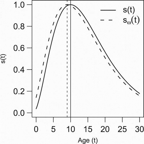
Figure 9. Gamma selectivity functions, s(t) and sω(t)=s(t+1). Vertical lines indicate the age at maximum selection.

Figure 9. Gamma selectivity functions, s(t) and sω(t)=s(t+1). Vertical lines indicate the age at maximum selection.

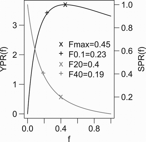
Figure 10. Yield and spawner per recruit curves and four fishing mortality RPs, Fmax,F0.1,F20%, and F40% for s(t) in Figure .

Figure 10. Yield and spawner per recruit curves and four fishing mortality RPs, Fmax,F0.1,F20%, and F40% for s(t) in Figure 9.

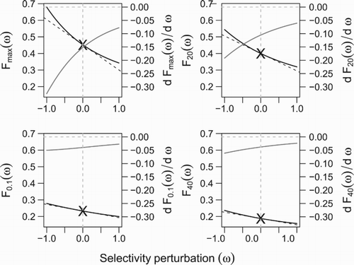
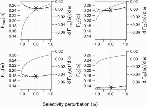
Figure 11. Solid black curves are values of F RPs for perturbed values of the selectivity function, sω(t)=s(t+ω) in Figure . Solid grey curves are the local slopes. Reference lines (grey dashed) indicate the local slope at ω=0.

Figure 11. Solid black curves are values of F RPs for perturbed values of the selectivity function, sω(t)=s(t+ω) in Figure 9. Solid grey curves are the local slopes. Reference lines (grey dashed) indicate the local slope at ω=0.

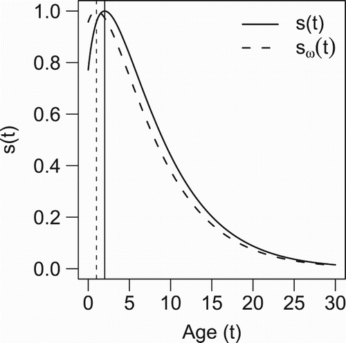
Figure 12. Gamma selectivity functions, s(t) and sω(t)=s(t+1). Vertical lines indicate the age at maximum selection.

Figure 12. Gamma selectivity functions, s(t) and sω(t)=s(t+1). Vertical lines indicate the age at maximum selection.

Figure 13. Yield and spawner per recruit curves and four fishing mortality RPs, Fmax,F0.1,F20%, and F40% for s(t) in Figure .

Figure 13. Yield and spawner per recruit curves and four fishing mortality RPs, Fmax,F0.1,F20%, and F40% for s(t) in Figure 12.

Figure 14. Solid black curves are values of F RPs for perturbed values of the selectivity function, sω(t)=s(t+ω) in Figure . Solid grey curves are the local slopes. Reference lines (grey dashed) indicate the local slope at ω=0.

Figure 14. Solid black curves are values of F RPs for perturbed values of the selectivity function, sω(t)=s(t+ω) in Figure 11. Solid grey curves are the local slopes. Reference lines (grey dashed) indicate the local slope at ω=0.