The balance simplex in non-competitive 2-species scaled Lotka–Volterra systems

Figures & data

Figure 1. A general diagram of a carrying simplex (left) and balance simplex (right) in red. The diagonal blue line is the unit simplex and the orange points are steady states of the system. The grey curves are solution trajectories of the system.

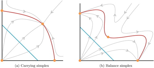
Figure 2. Phase plots of two species scaled Lotka–Volterra systems in the $x_1{x}_2$-plane. These four plots cover the generic qualitative dynamics of the system with different interspecific interaction coefficients (α and β). The orange points are the steady states of the system and the arrows show how solution trajectories evolve over time. ${}^{\ast }$Note (a) does not apply to the strongly co-operative case ($\alpha ,\beta <0$ and $\alpha \beta \ge 1$) where all positive solutions are unbounded.

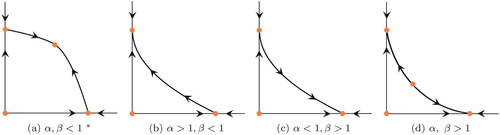
Figure 3. The parameter space $(\alpha ,\beta )$ with the different cases shown, each extending to infinity. Note that in the region of unbounded dynamics (both $\alpha ,\beta <0$ and $\alpha \beta \ge 1$), the balance simplex does not exist.

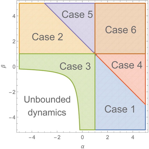
Table 1. The valid ranges in T for which we can use the solutions $R_1\left(T\right)$ and $R_2\left(1/T\right)$ in different parameter cases α and β. The remaining case (case 6) where both $\alpha ,\beta >1$ uses a slightly different solution and will be discussed later. A region plot of these cases can be found in Figure 3.

	$R_1\left(T\right)$	$R_2\left(T\right)$
Case 1:  $\beta <1,1<\alpha <2-\beta$	$[0,\mathrm{\infty })$	–
Case 2:  $\alpha <1,1<\beta <2-\alpha$	–	$[0,\mathrm{\infty })$
Case 3:  $\alpha ,\beta <1$ and $\alpha \beta <1$	$[0,T^{\ast }]$	$[T^{\ast },\mathrm{\infty })$
Case 4:  $\beta <1,1<2-\beta <\alpha$	$[0,\mathrm{\infty })$	–
Case 5:  $\alpha <1,1<2-\alpha <\beta$	–	$[0,\mathrm{\infty })$

Figure 4. Phase plots of two species scaled Lotka–Volterra systems with different interspecific interaction coefficients (α and β). Here (a) and (b) are competitive systems, (c) is a co-operative system and (d) is an example of predation. In these plots, the solutions $R_1\left(T\right)$ (dashed, orange) and $R_2\left(T\right)$ (solid, green) only meet at the interior steady state $x^{\ast }$.

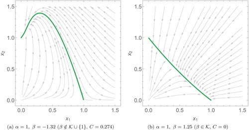
Figure 5. Phase plots of two species scaled Lotka–Volterra systems with different interspecific interaction coefficients (α and β). Here, (a) is an example of predation where we only need to use one solution, $R_1\left(T\right)$ (dashed, orange). (b) is a competitive system, using the solutions $R_1^{\ast }\left(T\right)$ (solid, black) and $R_2^{\ast }\left(T\right)$ (dashed and dotted, red).

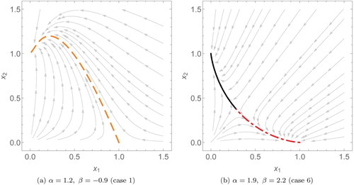
Figure A.1. Phase plots of two species scaled Lotka–Volterra systems where one of the interspecific interaction coefficients, α (without loss of generality), is equal to 1. The solid green curve is the balance simplex, connecting both axial steady states.