Figures & data
Figure 1. Existence region (red) for at
.
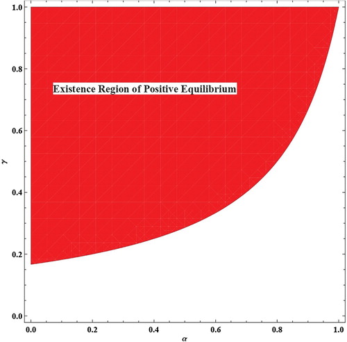
Figure 2. Topological classification of for
and
.
![Figure 2. Topological classification of P0 for α∈[0,2] and γ∈[0,2].](/cms/asset/1b5965b2-d2e8-4561-b145-cf24a30c22d4/tjbd_a_1638976_f0002_oc.jpg)
Figure 3. Topological classification of for
,
and
.
![Figure 3. Topological classification of P1 for α∈[0,1], β∈[0,200] and γ=0.995.](/cms/asset/98b5b6c9-7b9e-464e-9847-f74b8f75fd44/tjbd_a_1638976_f0003_oc.jpg)
Figure 4. Topological classification of for
,
and
.
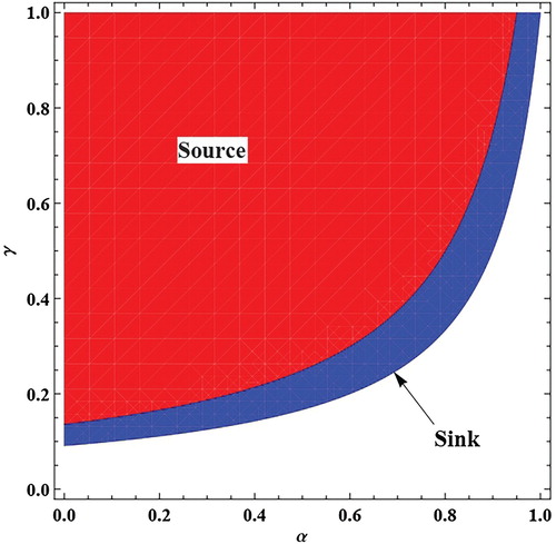
Figure 5. Bifurcation diagrams and MLE for system (Equation1(1)
(1) ) with
,
,
and
: (a) bifurcation diagram for
, (b) bifurcation diagram for
and (c) MLE.
![Figure 5. Bifurcation diagrams and MLE for system (Equation1(1) xn+1=xnα(1+yn2)+βxn,yn+1=γyn(1+xn),(1) ) with α=0.99, β=0.008, γ∈[0.2,0.7] and (x0,y0)=(1.25,0.001): (a) bifurcation diagram for xn, (b) bifurcation diagram for yn and (c) MLE.](/cms/asset/82e28a26-63d3-4307-99ad-29dcb487b7e3/tjbd_a_1638976_f0005_oc.jpg)
Figure 6. Bifurcation diagrams and MLE for system (Equation1(1)
(1) ) with
,
,
and
: (a) bifurcation diagram for
, (b) bifurcation diagram for
and (c) MLE.
![Figure 6. Bifurcation diagrams and MLE for system (Equation1(1) xn+1=xnα(1+yn2)+βxn,yn+1=γyn(1+xn),(1) ) with α=0.2, β=0.5, γ∈[0.45,0.95] and (x0,y0)=(0.78,1.426): (a) bifurcation diagram for xn, (b) bifurcation diagram for yn and (c) MLE.](/cms/asset/d9e22d06-97ca-4dc8-ace6-aa122274b477/tjbd_a_1638976_f0006_oc.jpg)
Figure 7. Phase portraits of system (Equation1(1)
(1) ) for
,
,
and with different values of γ: (a) phase portrait for
, (b) phase portrait for
, (c) phase portrait for
and (d) phase portrait for
.
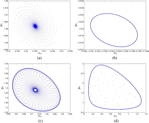
Figure 8. Bounded stability region for system (Equation24(24)
(24) ).
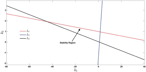
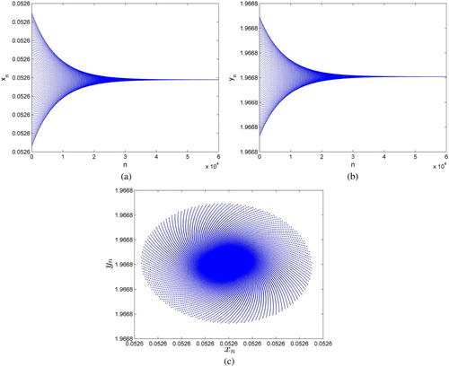
Figure 9. Plots for system (Equation25(25)
(25) ) with
and
: (a) plot for
, (b) plot for
and (c) phase portrait.