Global dynamics of a tuberculosis model with fast and slow progression and age-dependent latency and infection

Figures & data

Table 1. Definitions of the parameters and symbols in the system (3(3) $\begin{array}{rl}\dot{S}(t)& =A-{\mu }_{S}S(t)-S(t){\int }_0^{\mathrm{\infty }}\beta (a)i(a,t)\mathrm{d}a,\\ {\displaystyle \frac{\mathrm{\partial }e(\theta ,t)}{\mathrm{\partial }t}+{\displaystyle \frac{\mathrm{\partial }e(\theta ,t)}{\mathrm{\partial }\theta }}}& =-(\mu (\theta )+\epsilon (\theta ))e(\theta ,t),\theta >0,\\ {\displaystyle \frac{\mathrm{\partial }i(a,t)}{\mathrm{\partial }t}+{\displaystyle \frac{\mathrm{\partial }i(a,t)}{\mathrm{\partial }a}}}& =-\nu (a)i(a,t),a>0\end{array}$(3) ).

Parameters	Description
A	The recruitment rate
${\mu }_S$	Per capita natural death rate of the susceptible population
θ	The duration for which individuals have been in the latently infected class
a	Age of infection, i.e. the time that has lapsed since the individual became infectious
$\mu (\theta )$	The rate at which individuals who have been in the latently infected class for duration θ are removed
$\epsilon (\theta )$	The rate at which individuals who have been in the latently infected class for duration θ progress to the active infectious class
$\beta (a)$	The transmission coefficient of active infectious individuals at age of infection a
$\nu (a)$	The natural and disease-induced death rate of individuals who have been in the active infectious class for duration a
p	The proportion of the newly infected to develop tuberculosis directly
1−p	The proportion of the newly infected to enter the latent class

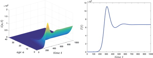
Figure 1. The temporal solution found by numerical integration of system (3(3) $\begin{array}{rl}\dot{S}(t)& =A-{\mu }_{S}S(t)-S(t){\int }_0^{\mathrm{\infty }}\beta (a)i(a,t)\mathrm{d}a,\\ {\displaystyle \frac{\mathrm{\partial }e(\theta ,t)}{\mathrm{\partial }t}+{\displaystyle \frac{\mathrm{\partial }e(\theta ,t)}{\mathrm{\partial }\theta }}}& =-(\mu (\theta )+\epsilon (\theta ))e(\theta ,t),\theta >0,\\ {\displaystyle \frac{\mathrm{\partial }i(a,t)}{\mathrm{\partial }t}+{\displaystyle \frac{\mathrm{\partial }i(a,t)}{\mathrm{\partial }a}}}& =-\nu (a)i(a,t),a>0\end{array}$(3) ) with the boundary conditions (4(4) $\begin{array}{rl}e(0,t)& =(1-p)S(t){\int }_0^{\mathrm{\infty }}\beta (a)i(a,t)\mathrm{d}a,\\ i(0,t)& =pS(t){\int }_0^{\mathrm{\infty }}\beta (a)i(a,t)\mathrm{d}a+{\int }_0^{\mathrm{\infty }}\epsilon (\theta )e(\theta ,t)\mathrm{d}\theta ,\end{array}$(4) ) and the initial condition $S(0)=1.4\times {10}^7,e_0(\theta )={\mathrm{e}}^{-\theta },i_0(a)={\mathrm{e}}^{-a}$, and the parameters given in (88(88) $\beta (a)=\{\begin{array}{ll}3\times {10}^{-7}{\mathrm{person}}^{-1}{\mathrm{year}}^{-1},& a<1,\\ 1.5\times {10}^{-7}{\mathrm{person}}^{-1}{\mathrm{year}}^{-1},& a\ge 1.\end{array}$(88) ) and (89(89) $\begin{array}{rl}& A=2\times {10}^5\mathrm{people}\mathrm{yea}{\mathrm{r}}^{-1},{\mu }_S=1/70\mathrm{yea}{\mathrm{r}}^{-1},\nu (a)=0.1612\mathrm{yea}{\mathrm{r}}^{-1},\\ & p=0.05,\mu (\theta )=1/70\mathrm{yea}{\mathrm{r}}^{-1},\epsilon (\theta )=0.00256\mathrm{yea}{\mathrm{r}}^{-1}.\end{array}$(89) ).