Melnikov analysis of chaos in a simple SIR model with periodically or stochastically modulated nonlinear incidence rate

Figures & data

Figure 1. The spectral density of bounded noise for $b_4=1,{\mathrm{\Omega }}_2=1$. (a) $\sigma =0.1$. (b) $\sigma =0.5$. (c) $\sigma =1$ and (d) $\sigma =2$.

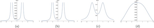
Figure 2. Phase portraits of the system (31(31) $\begin{array}{rl}\frac{\mathrm{d}x}{\mathrm{d}\tau }& =y,\\ \frac{\mathrm{d}y}{\mathrm{d}\tau }& =-c^2+x^2+ϵ(b_{1}y+xy-4b_3\sin ({\mathrm{\Omega }}_1\tau )-4b_4\xi (\tau ))+o({ϵ}^2),\end{array}$(31) ) for $b_3=0,b_4=0$.(a) $b_1=2,b_2=3/2$. (b) $b_1=2,b_2=5/2$ and (c) $b_1=2,b_2=3$

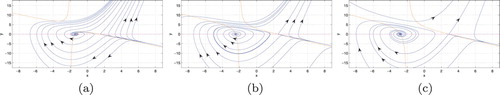
Figure 3. Phase portrait and potential of the system (32(32) $\begin{array}{rl}\frac{\mathrm{d}x}{\mathrm{d}\tau }& =y,\\ \frac{\mathrm{d}y}{\mathrm{d}\tau }& =-c^2+x^2=-(4b_2-b_1^2)+x^2,\end{array}$(32) ) for $b_1=0,b_2=1$. (a) Phase portrait. (b) Potential.

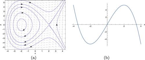
Figure 4. The homoclinic bifurcation curve for Smale chaos in the $({\mathrm{\Omega }}_1,b_3)$ plane. (a) $b_1=0,b_2=1$ and (b) $b_1=0,b_2=2$.

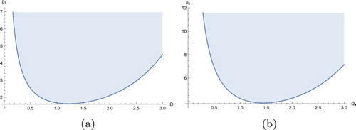
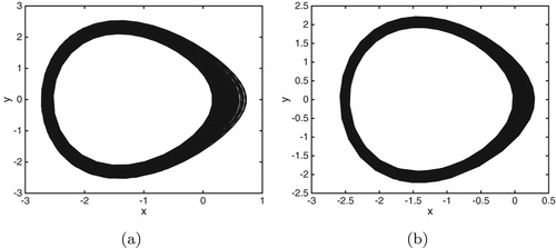
Figure 5. Phase portrait with $b_1=0,{\mathrm{\Omega }}_1=2,ϵ=0.00001$ and initial value: $x(0)=0.1,y(0)=0.2$. (a) $b_2=1,b_3=3$ and (b) $b_2=2,b_3=5$.

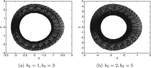
Figure 6. Upper bound for possible chaotic domain due to homoclinic bifurcation $(\mathrm{\Psi }=0)$ with ${\mathrm{\Omega }}_1=1,{\mathrm{\Omega }}_2=2,b_2=1$. (a) Upper surface in $(b_3,b_4,b_1)$ space. (b) Upper bound in $(b_3,b_1)$ plane with $b_4=1$ and (c) Upper bound in $(b_4,b_1)$ plane with $b_3=0.2$.

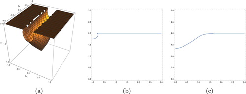
Figure 7. (a) Bifurcation curve $({38}^{\prime })$ for the homoclinic orbits ${\mathrm{\Gamma }}_{hom}$. Here $b_1=2,b_2=3/2,b_3=1,{\mathrm{\Omega }}_1=1/3$ and ${\mathrm{\Omega }}_2=\sqrt{3}$; (b) Phase portrait for (31(31) $\begin{array}{rl}\frac{\mathrm{d}x}{\mathrm{d}\tau }& =y,\\ \frac{\mathrm{d}y}{\mathrm{d}\tau }& =-c^2+x^2+ϵ(b_{1}y+xy-4b_3\sin ({\mathrm{\Omega }}_1\tau )-4b_4\xi (\tau ))+o({ϵ}^2),\end{array}$(31) ) with $b_1=2,b_2=3/2,b_3=1,b_4=2,{\mathrm{\Omega }}_1=1/3,{\mathrm{\Omega }}_2=\sqrt{3},ϵ=0.00001$ and initial value: $x(0)=0.1,y(0)=0.2$.

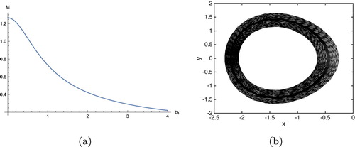
Figure 8. The surface in $(b_1,b_2,t_0)$ plane for $I_1=0$.

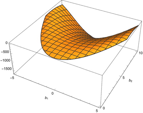
Figure 9. The threshold amplitude $b_4$ of bounded noise excitation for the onset of chaos in system (31(31) $\begin{array}{rl}\frac{\mathrm{d}x}{\mathrm{d}\tau }& =y,\\ \frac{\mathrm{d}y}{\mathrm{d}\tau }& =-c^2+x^2+ϵ(b_{1}y+xy-4b_3\sin ({\mathrm{\Omega }}_1\tau )-4b_4\xi (\tau ))+o({ϵ}^2),\end{array}$(31) ) with $b_3=0,b_1=2,b_2=3/2,{\mathrm{\Omega }}_2=2$. (a) $\sigma \in [0,3];(b)\sigma \in [0,1]$.

Figure 10. Phase portraits of the system (31(31) $\begin{array}{rl}\frac{\mathrm{d}x}{\mathrm{d}\tau }& =y,\\ \frac{\mathrm{d}y}{\mathrm{d}\tau }& =-c^2+x^2+ϵ(b_{1}y+xy-4b_3\sin ({\mathrm{\Omega }}_1\tau )-4b_4\xi (\tau ))+o({ϵ}^2),\end{array}$(31) ) with $b_3=0,b_1=2,b_2=3/2,{\mathrm{\Omega }}_2=2$ and $ϵ=0.00001$. (a) $b_4=7.5,\sigma =0.5$ with initial value: $x(0)=0.1,y(0)=0.2$. (b) $b_4=10,\sigma =2$ with initial value: $x(0)=-0.1,y(0)=0.2$.