Impulsive releases of sterile mosquitoes and interactive dynamics with time delay

Figures & data

Figure 1. Schematic graph of release function $g\left(t\right)$ with the assumption $\overline{T}<T<2\overline{T}$ for $k\ge 1$.

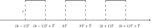
Figure 2. Schematic graph of release function $g\left(t\right)$ for $k\ge 2$ with the assumption $T<\overline{T}<2T$.

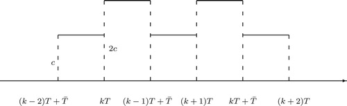
Figure 3. The parameters are given in (9(9) $a=50,{\mu }_0=0.3,\mu =0.2,\xi =0.1,\tau =9,$(9) ) such that the release threshold $g^{\ast }=7.4304$. We assume that the sterile mosquitoes are released at T = 10 and T = 5, respectively. The solutions for T = 10 are shown in the left figure, where we let c = 10, 15, and 20, and the corresponding solutions are in blue, red, and black, respectively, none of which approaches zero. The solutions for T = 5 are shown in the right figure, where we have c = 10 and $y\left(0\right)=4$, 8, 14, and the corresponding solutions are in blue, red, and black, respectively, all of which approach zero.

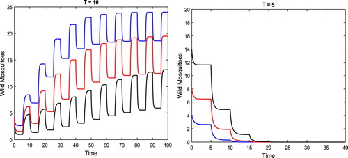
Figure 4. Parameters are given in (9(9) $a=50,{\mu }_0=0.3,\mu =0.2,\xi =0.1,\tau =9,$(9) ) and the release times are T = 10 and T = 5, respectively. The results with different release amounts of sterile mosquitoes c are compared. For T = 10, we gradually increase c from $12,18,25$, to 28. The corresponding solutions w with the same initial values are shown in the left figure. For T = 5, the release amounts c are gradually increased from $3,5,6$, to 7. The corresponding solutions w with the same initial values are shown in the right figure.

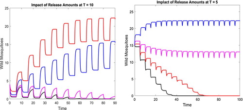
Table 1. Summary table for $\overline{T}<\tau <T<\overline{T}+\tau$.

	$kT\le t<kT+\overline{T}$
	$kT\le t<(k-1)T+\overline{T}+\tau$	$(k-1)T+\overline{T}+\tau \le t<kT+\overline{T}$
$g\left(t\right)$	c
$g(t-\tau )$	c	0
	$kT+\overline{T}<t\le (k+1)T$
	$kT+\overline{T}<t\le kT+\tau$	$kT+\tau <t<(k+1)T$
$g\left(t\right)$	0
$g(t-\tau )$	0	c

Figure 5. With parameters given in (13(13) $a=20,{\mu }_0=0.3,\mu =0.2,\xi =0.1,\tau =9,$(13) ), $c=5<g^{\ast }=5.1637$, and condition (10(10) $\overline{T}<\tau <T<\overline{T}+\tau .$(10) ) holds. There exists a positive 10-periodic solution, between $w_1^{+}=8.2477$ and $w_3^{+}=22.4913$, as shown in the figure.

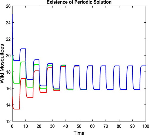
Table 2. Summary table for $T<\overline{T}<\tau <2T$ and $\tau +\overline{T}<3T$.

	$0<t\le T$	$T\le t<\overline{T}$	$\overline{T}<t\le 2T$
			$\overline{T}<t\le \tau$	$\tau <t\le 2T$
$g\left(t\right)$	c	2c	c
$g(t-\tau )$	0	0	0	c
	For $k\ge 1$:
	$(k+1)T\le t<kT+\overline{T}$
$g\left(t\right)$	2c
$g(t-\tau )$	c
	$kT+\overline{T}\le t<(k+2)T$
	$kT+\overline{T}\le t<kT+\tau$	$kT+\tau \le t<(k-1)T+\overline{T}+\tau$	$(k-1)T+\overline{T}+\tau \le t<(k+2)T$
$g\left(t\right)$	c
$g(t-\tau )$	c	2c	c

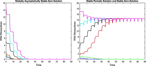
Figure 6. With parameters given in (18(18) $a=20,{\mu }_0=0.3,\mu =0.2,\xi =0.1,\tau =7,$(18) ), condition (14(14) $T<\overline{T}<\tau <2T,\tau +\overline{T}<3T.$(14) ) holds. For $c=6>g^{\ast }=5.1637$, since $\underset{t\in (0,\mathrm{\infty })}{inf}g\left(t\right)=6>g^{\ast }$, the zero solution is globally asymptotically stable as shown in the left figure. For $c=2.5<g_2^{\ast }=2.5818$, there exists a periodic solution which seems asymptotically stable as shown in the right figure.