The role of asymptomatic class, quarantine and isolation in the transmission of COVID-19

Figures & data

Figure 1. Schematic diagram of the model (2(2) $\begin{array}{rl}\frac{\mathrm{d}S}{\mathrm{d}t}& =\mathrm{\Pi }+\xi Q_S-(\lambda +\mu +ϵ)S\\ \frac{\mathrm{d}{Q}_S}{\mathrm{d}t}& =ϵS-(\xi +\mu )Q_S\\ \frac{\mathrm{d}E}{\mathrm{d}t}& =\rho \lambda S-({\kappa }_E+\sigma +\mu )E\\ \frac{\mathrm{d}{Q}_E}{\mathrm{d}t}& ={\kappa }_{E}E-({\omega }_E+\nu +\mu )Q_E\\ \frac{\mathrm{d}I}{\mathrm{d}t}& =\sigma E+\nu Q_E-({\delta }_I+\tau +\mu +\gamma )I\\ \frac{\mathrm{d}A}{\mathrm{d}t}& =(1-\rho )\lambda S-({\kappa }_A+{\theta }_A+\mu )A\\ \frac{\mathrm{d}{Q}_A}{\mathrm{d}t}& ={\kappa }_{A}A-({\omega }_A+\mu )Q_A\\ \frac{\mathrm{d}{Q}_I}{\mathrm{d}t}& =\tau I+{\omega }_E{Q}_E-(\theta +{\delta }_Q+\mu )Q_I\\ \frac{\mathrm{d}R}{\mathrm{d}t}& =\theta Q_I+\gamma I+{\theta }_{A}A+{\omega }_A{Q}_A-\mu R\end{array}$(2) ).

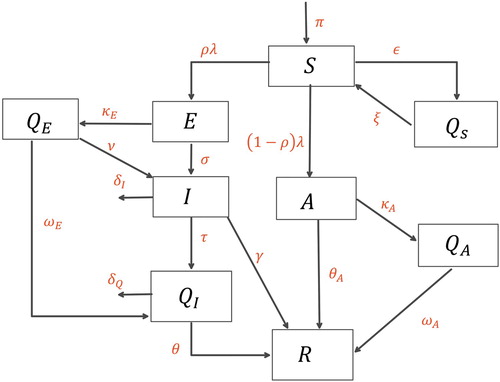
Table 1. Description of the variables of the model.

Variable	Description
N	Total population
S	Susceptible individuals
E	Individuals exposed to corona virus
$Q_S$	Individuals self quarantined
I	Individuals infected with corona virus
A	Asymptomatic individuals
$Q_E$	Quarantine of exposed individuals
$Q_I$	Isolated individuals
$Q_A$	Quarantine of asymptomatic individuals
R	Recovered from corona virus

Table 2. Description of the parameters of the model.

Parameters	Description	Values
Π	Recruitment rate of humans	100	Assumed
μ	Natural death rate of humans	60 years	Assumed
${\delta }_I$	Disease-induced death rate individuals	$0.065{\mathrm{day}}^{-1}$	Estimated
${\delta }_Q$	Disease-induced death rate of isolated individuals	$0.04{\mathrm{day}}^{-1}$	Assumed
ν	Rate of infectious of exposed quarantined individuals	0.4	Assumed
$\frac{1}{\sigma }$	Incubation rate of susceptible individuals	3−5 days	[7,8]
$\frac{1}{\gamma }$	Recovery rate of infected individuals	10 days	[7,8]
β	Effective contact rate	0.4−0.9	[7]
ρ	Probability of getting exposed to covid-19	$40\mathrm{\%}=0.4$	[7]
τ	Isolation rate of infected individuals	0.2	[7]
${\kappa }_E$	Quarantine rate of exposed individuals	0.4	Assumed
${\kappa }_A$	Quarantine rate of asymptomatic individuals	0.4	Assumed
${\omega }_E$	Isolation rate of exposed quarantined individuals	0.1	Assumed
${\omega }_A$	Recovery rate of exposed asymptomatic individuals	0.1	[7,8]
${\theta }_A$	Recovery rate of asymptomatic individuals	0.1	[7,8]
θ	Recovery rate of isolated individuals	0.05	[7,8]
ε	Self quarantine rate of susceptible individuals	0.5	Assumed
ξ	Waning rate of self quarantined individuals	0.4	Assumed
	to susceptible class
${\eta }_1$	Modification parameter for relative infectiousness	0.2	Assumed
	of isolated individuals
${\eta }_2$	Modification parameter for relative infectiousness	0.5	[7]
	of asymptomatic individuals
${\eta }_3$	Modification parameter for relative infectiousness	0.2	Assumed
	asymptomatic quarantined

Figure 2. Time Series Analysis. (a) ${\mathcal{R}}_0<1$. (b) ${\mathcal{R}}_0>1$.

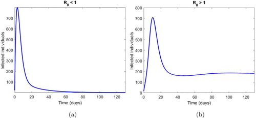
Figure 3. Contour graph of the self quarantine with rate of isolation and rate of isolation. (a) ε vs ${\mathcal{R}}_0$. (b) τ vs ${\mathcal{R}}_0$. (c) τ vs ε with $\beta =0.9$.

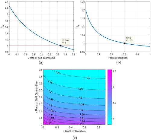
Figure 4. Sensitivity of the parameters.

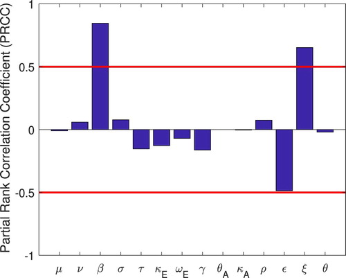
Figure 5. Uncertainty analysis. (a) Uncertainty of parameters, (b) Uncertainty of R₀.

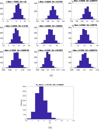
Figure 6. Optimal control of τ. (a) Cost comparison fro τ. (b) Infected pop comparison. (c) Control strategies for τ.

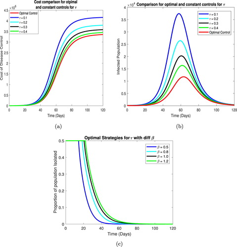
Figure 7. Optimal control for ε. (a) Cost comparison for ε. (b) Infected pop comparison. (c)Control Strategies for ε.

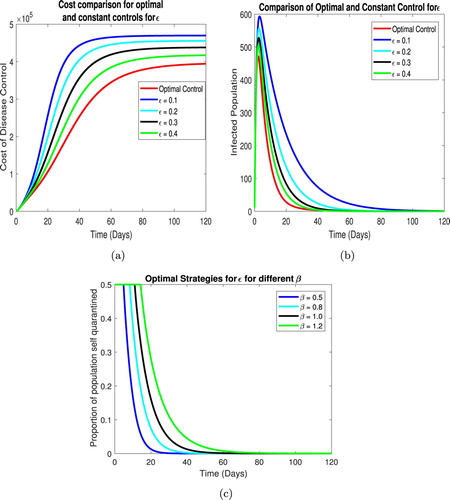
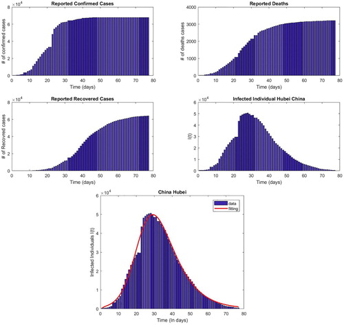
Figure 8. Reported data and parameter estimation.

Table 3. $R_0$ Estimates.

Parameter	Estimated values	$95\mathrm{\%}$ CI
β	1.248	1.2−1.3
γ	0.603	0.59−0.63
σ	0.546	0.52−0.57
δ	0.065	0.0047−0.1
${\mathcal{R}}_0$	1.8678	1.36−2.4

S. Eikenberry, M. Mancuso, E. Iboi, T. Phan, K. Eikenberry, Y. Kuang, E. Kostelich, and A. Gumel, To mask or not to mask: Modeling the potential for face mask use by the general public to curtail the COVID-19 pandemic, Infect. Dis. Model. 5 (2020), pp. 293–308.

 PubMedGoogle Scholar

N. Ferguson, D. Laydon, G. Nedjati Gilani, N. Imai, K. Ainslie, M. Baguelin, S. Bhatia, A. Boonyasiri, Z. Cucunuba Perez, G. Cuomo-Dannenburg, A. Dighe, I. Dorigatti, H. Fu, K. Gaythorpe, W. Green, A. Hamlet, W. Hinsley, L. Okell, S. Van Elsland, H. Thompson, R. Verity, E. Volz, H. Wang, Y.Wang, P. Walker, C. Walters, P. Winskill, C. Whittaker, C. Donnelly, S. Riley, and A. Ghani, Report 9: Impact of non-pharmaceutical interventions (Npis) to reduce COVID19 mortality and healthcare demand, 2020. [online] Hdl.handle.net. Available at http://hdl.handle.net/10044/1/77482 (accessed 2 May 2020).

 Google Scholar