A bifurcation theorem for Darwinian matrix models and an application to the evolution of reproductive life-history strategies

Figures & data

Figure 1. Two examples are shown for Equations (20(20) $\begin{array}{rl}x(t+1)& =[(b{s}_n-s_a)\exp (-w_0{u}^2\left(t\right))+s_a]\frac{x\left(t\right)}{1+c_{0}x\left(t\right)}\end{array}$(20) ) and (21(21) $\begin{array}{rl}u(t+1)& =(1-2w_0{\sigma }^2\frac{(b{s}_n-s_a)\exp (-w_0{u}^2\left(t\right))}{(b{s}_n-s_a)\exp (-w_0{u}^2\left(t\right))+s_a})u\left(t\right).\end{array}$(21) ) with parameter values $w_0=5,$ $w_1=5.5$, $c_0=1,$ $s_a=0.25,$ $s_n=0.5,$ and ${\sigma }^2=0.01$. In both cases $b>b_0=1/s_n=2$ and Theorem 4.1 implies the existence of a globally stable positive equilibrium with a semelparous trait component. (a) b = 5: four typical orbits in the x, u-phase plane are seen to approach the equilibrium $(x,u)=(1.5,0)$, and the adaptive landscape $L(v)$ has a global maximum at u = 0. (b) b = 40: four typical orbits x, u-phase plane are seen to approach a positive equilibrium $(x,u)=(19.0,0),$ and the adaptive landscape $L(v)$ has a local minimum at u = 0.

Figure 2. Shown are selected time snapshots of the adaptive landscape for the simulation in Figure 2(b) for the orbit with initial condition $(x(0),u(0))=(30,0.2)$. The trait component $u_t$ moves to the left towards the peak (not easily perceptible on the scale shown), but asymptotically arrives at a local minimum on the equilibrium landscape (shown in Figure 1(b)).

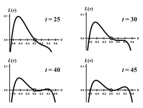
Figure 3. Two phase plane orbits are shown for the Darwinian model (5(5) $\begin{array}{rl}x(t+1)& ={r(x\left(t\right),u\left(t\right),v)|}_{v=u\left(t\right)}x\left(t\right)\end{array}$(5) )–(6(6) $\begin{array}{rl}u(t+1)& =u\left(t\right)+{\sigma }^2{\frac{\mathrm{\partial }\ln r(x\left(t\right),u\left(t\right),v)}{\mathrm{\partial }v}|}_{v=u\left(t\right)}.\end{array}$(6) )–(23(23) $r(b,x,u,v)=b{e}^{-w_0{v}^2}\frac{1}{1+c_0{e}^{-w_1(v-u)}x}{s}_n\frac{1+\rho a_0{u}^2{x}^q}{1+a_0{u}^2{x}^q}+s_a(1-e^{-w_0{v}^2})$(23) ) with parameters values $b=3.4,$ $w_0=1,$ $c_0=0.2,$ $w_1=1,$ $\rho =3,$ $a_0=0.2,$ $s_n=0.3,$ $s_a=0.9,$ $q=2,$ ${\sigma }^2=\mathrm{0.4.}$ Note that $b>b_0=1/s_n=10/3$ and hence the extinction equilibrium $(0,0)$ is unstable. The orbit with initial condition $(x(0),u(0))=(5,0)$ approaches the positive equilibrium $(x_1,u_1)=(0.096,0.093)$ (open square), which is the bifurcating equilibrium from the extinction equilibrium $(0,0)$ predicted by Theorem 4.2. The orbit with initial condition $(x(0),u(0))=(6,0)$ approaches a different equilibrium, namely. $(x_2,u_2)=(6.789,1.086)$ (open square). Both equilibrium trait values lie on global maxima of their respective adaptive landscapes $L(v)$ (open squares) and hence are ESS traits.

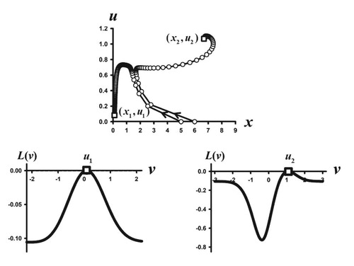
Figure 4. Two phase plane orbits are shown for the Darwinian model (5(5) $\begin{array}{rl}x(t+1)& ={r(x\left(t\right),u\left(t\right),v)|}_{v=u\left(t\right)}x\left(t\right)\end{array}$(5) )–(6(6) $\begin{array}{rl}u(t+1)& =u\left(t\right)+{\sigma }^2{\frac{\mathrm{\partial }\ln r(x\left(t\right),u\left(t\right),v)}{\mathrm{\partial }v}|}_{v=u\left(t\right)}.\end{array}$(6) )–(23(23) $r(b,x,u,v)=b{e}^{-w_0{v}^2}\frac{1}{1+c_0{e}^{-w_1(v-u)}x}{s}_n\frac{1+\rho a_0{u}^2{x}^q}{1+a_0{u}^2{x}^q}+s_a(1-e^{-w_0{v}^2})$(23) ) with the same parameters values as in Figure 3 except that b has been changed to b = 3.2. Since $b<b_0=1/s_n=10/3$ the extinction equilibrium $(x_1,u_1)=(0,0)$ is stable, as is illustrated by the orbit with initial condition $(x(0),u(0))=(8,0)$. However, the orbit with initial condition $(x(0),u(0))=(9,0)$ approaches a positive equilibrium $(x_2,u_2)=(6.036,1.065)$, whose trait component is an ESS as the accompanying graph of the adaptive landscape $L(v)$ shows.

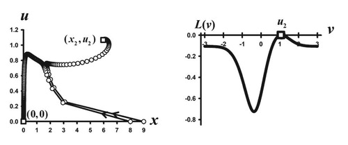
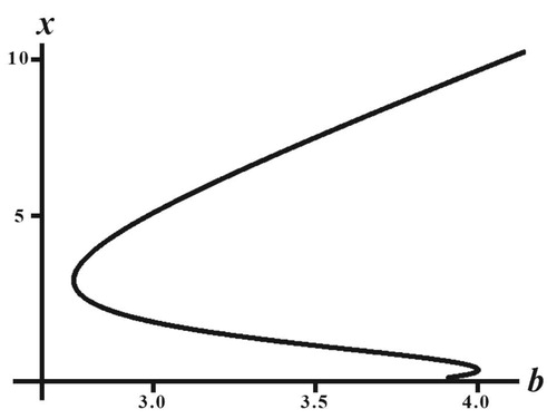
Figure 5. Shown is a plot of the Equation (24(24) $b{e}^{-w_0{u}^2}\frac{1}{1+c_{0}x}{s}_n\frac{1+\rho a_0{u}^2{x}^2}{1+a_0{u}^2{x}^2}+s_a(1-e^{-w_0{u}^2})=1.$(24) ) in the $(b,x)$-plane with parameter values used in Figures 3 and 4 and $u=1.$