Figures & data
Figure 1. Linked-data-based GIS workflow architecture, highlighting the role of workflow typing and enrichment on the web with local GIS.
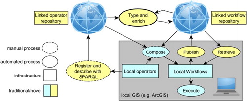
Table 1. Types of spatio-temporal references.
Table 2. Types of functional concepts.
Table 3. GIS-specific types of references.
Figure 2. Distinction between data items, supports, and measures.
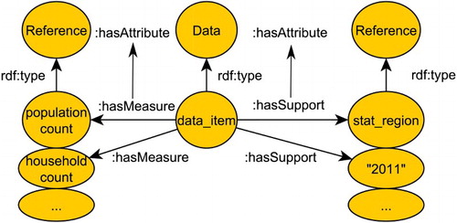
Table 4. GIS data types.
Figure 3. Concepts for typing geoprocessing workflows. Provenance relations are denoted by the property of. Rectangles: function classes.
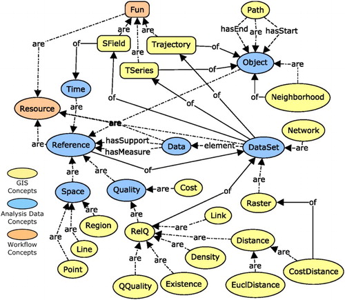
Figure 4. Provenance graph of GIS types derived from the concepts ‘field’ and ‘object’. Black arrows link concepts to predecessors in the geoprocessing chain. Concepts indirectly represented as data are denoted by dotted boxes (e.g. fields are indirectly represented by rasters).
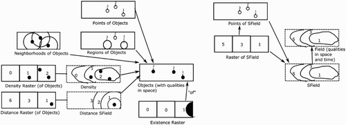
Figure 5. Linked data pattern (classes and properties) for modeling workflows. Workflows are linked to their subgraphs via reified statements. Operations are functions applied to inputs and producing outputs, resources are used to build a workflow (may also be functions). The of relation links resources to their origins.
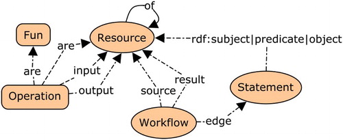
Figure 6. Example of usage of the workflow pattern wf to add explicit and implicit (dotted) semantic structures between inputs and outputs in a geoprocessing workflow for point interpolation.
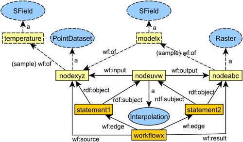
Table 5. Vocabularies used in this article.
Figure 7. Backtracking from sources to results to enrich a workflow. For each operation, we first type inputs (if not already present), then outputs, and then link outputs to inputs, and then proceed to the next operation.
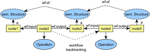
Figure 8. Schematic map illustration of least-cost path integration. Arrows between RDF types stand for links between their instances.
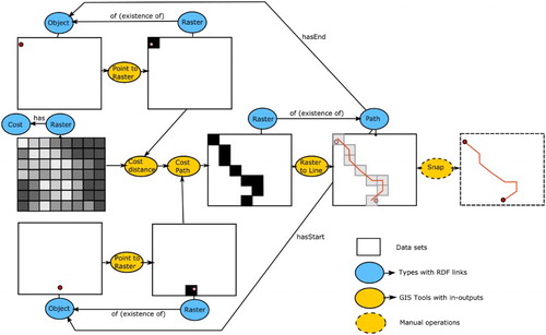
Figure 9. Workflow #1: ModelBuilder workflow to calculate the change in night lights in China. The blue ovals are input datasets, yellow rectangles indicate operations, and the green ovals are output datasets.
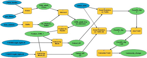
Figure 10. Workflow #1: Variation in average nocturnal luminosity over China from 1993 to 2013. Courtesy of Andy Bartle (Birkbeck, University of London).
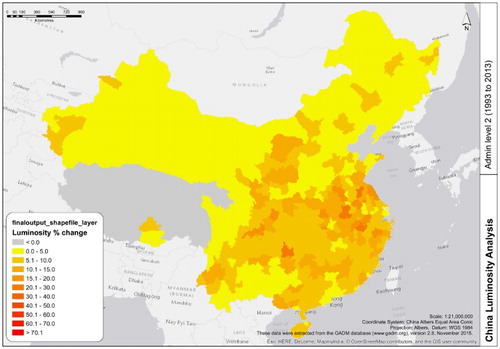
Figure 11. Workflow #2: ModelBuilder workflow of planning a new highway (myroute) connecting two highway exits (endraster, beginraster) based on avoiding built environment, nature areas, and other landuse classes. The latter objects enter the model in terms of a cost surface on which a least-cost path is computed. Blue ellipses denote root data sets, green ones intermediate data, and yellow boxes denote function applications.
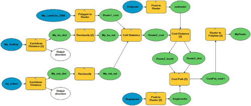
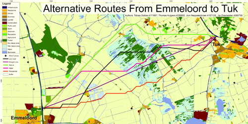
Figure 12. A map of different road alternatives generated based on the workflow of . Courtesy of Tobias Dobbe, Jorn Neppelenbroek, Thomas Kuijpers and Jip Zinsmeister.