
Figures & data
Figure 1. Study area and the locations of data for model training and validation. The Shuttle Radar Topography Mission (SRTM) elevation data (Farr and Kobrick Citation2000) are used as the base map.
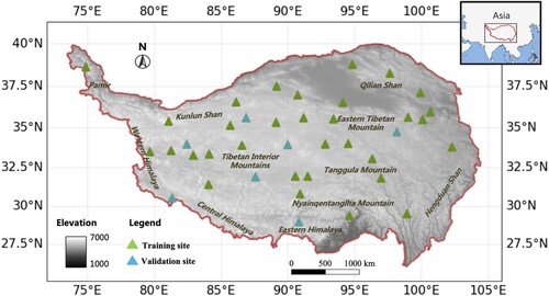
Figure 2. Space-time distribution of the acquired Sentinel-1 images. a. Temporal distribution of acquired Sentinel-1 images in ascending and descending tracks. The high transparency of the color represents that fewer images are collected on a specific day of the year. b. Spatial distribution of ascending observations. c. Spatial distribution of descending observations.
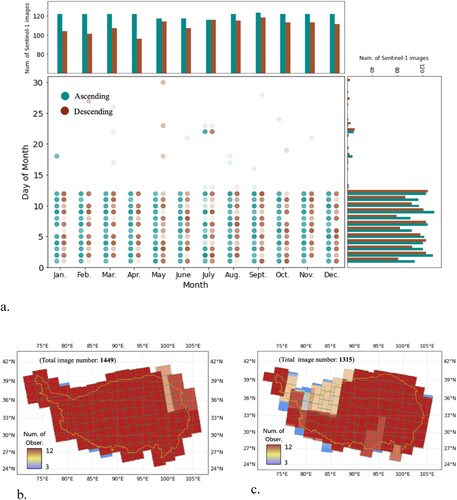
Figure 3. Demonstration of the Sentinel-1 SAR image-based surface water dataset. Sentinel-1 scene is visualized with a color composite of the VV band (R)-VH band (G)-VV band (B), and the reference Sentinel-2 scene is visualized with a false-color composite of NIR (R)-Red (G)-Green (B).
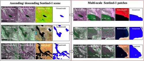
Figure 4. The workflow of our study. GEE: Google Earth Engine; S1: Sentinel-1 satellite.
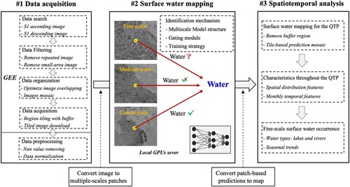
Figure 5. Structure of the proposed gated multiscale ConvNet.
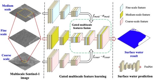
Figure 6. Gating modules for medium-scale and coarse-scales features, respectively.
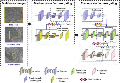
Table 1. ConvNet structure in this study. ‘In’, ‘Ex’, and ‘Out’ represent the numbers of input, exchange, and output channels, respectively.
Table 2. Layers of the Dsample and Upsample modules.
Table 3. Accuracies of the surface water map derived by GMNet and the comparison methods.
Table 4. Accuracies of the surface water map derived by GMNet for the validation sites.
Figure 7. Comparison of model performances during model training. (a) and (b) correspond to validation accuracy and model loss value metrics, respectively.
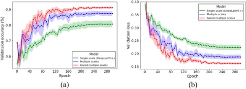
Figure 8. Illustrations of surface water mapping for the easily recognized scene, complex scene, and large-size water body scene. Panels a, f and k are the Sentinel-1 images for the three scenes. The green and red boxes represent a larger-scale scene and the location of the visualized scene in the larger-scale scene. Panels b, g and l are the Sentinel-2 images used for references. Panels c, h and m are the results derived by the traditional single-scale deep learning model. Panels d, i and n are the results derived by the multiscale deep learning model. Panels e, j and o are the results derived by the gated multiscale deep learning model.
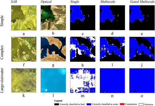
Figure 9. Comparison among models with training on ascending images only, descending images only, and combined ascending/descending images.
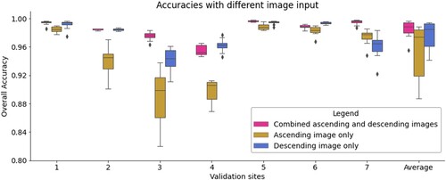
Figure 10. Comparisons of the surface water maps for validation site 3 that are derived from the trained models with different Sentinel-1 image acquisitions. a and f are Sentinel-1 ascending images; b and g are Sentinel-1 descending images; c and h are water maps derived from the trained model with ascending images only. d and i are water maps derived from the trained model with descending images only. Finally, e and j are water maps derived from the trained model with both ascending and descending images.
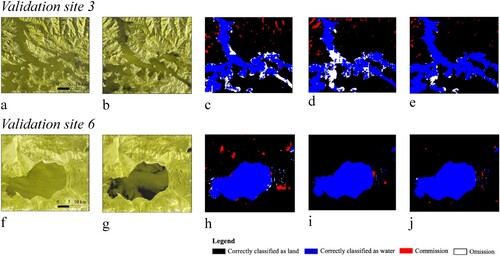
Figure 11. Monthly surface water area statistics for the QTP.
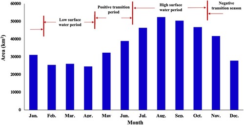
Figure 12. Spatial heterogeneity of the monthly surface water in the QTP region. a. the spatially resolved monthly surface water maps, and b. the surface water fluctuation map for the QTP region. The fluctuation is quantified by using the standard deviation metric.
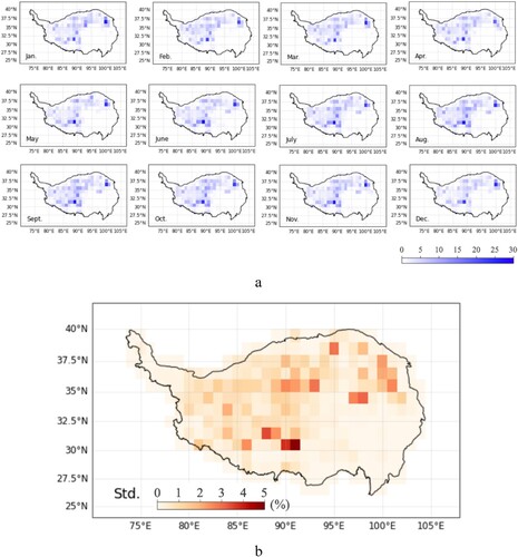
Figure 13. The dynamic surface water features of hydrological basins in the QTP region. a and b represent the surface water percentages of the hydrological basins in the dry season and wet season, respectively. c shows the standard deviation of the surface water areas in each hydrological basin. d, e, and f corresponding to local sites in Inner Tibetan Plateau, Yellow, and Yangtze basins, respectively. L8 and S2 represent the Landsat 8 and Sentinel-2 optical images, respectively.
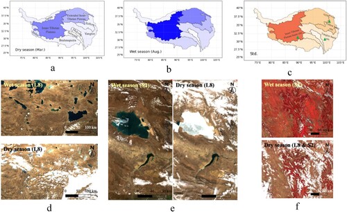
Figure 14. Surface water occurrence map in the QTP region.
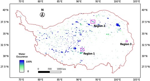
Figure 15. Surface water occurrence map for the selected region 1. The green and orange circles represent mutable and stable regions, respectively.
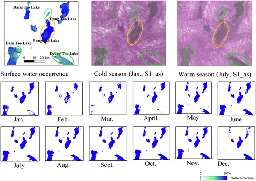
Figure 16. Surface water occurrence map for the selected region 3. The green circle labels a mutable region.
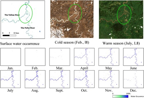
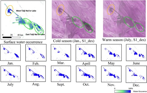
Figure 17. Surface water occurrence map for the selected region 2. The green and orange circles represent mutable and stable regions, respectively.
Data availability statement
The Sentinel-1 imagery used in this study is available from the Copernicus Data Space Ecosystem https://scihub.copernicus.eu/ and in Google Earth Engine https://earthengine.google.com/. The monthly surface water dataset generated in this study are available from https://doi.org/10.5281/zenodo.7768932.