Ice bottom evolution derived from thermistor string-based ice mass balance buoy observations

Figures & data

Figure 1. Deployment status of Snow and Ice Mass Balance Apparatus (SIMBA) and positions during deployment. (a) The Arctic Ocean, photo by Anne Bublitz (AWI), (b) the boreal Lake Orajärvi, photo by Bin Cheng (FMI), and (c) the Baltic Sea, photo by Pekka Kosloff (FMI). The yellow box represents the SIMBA’s main case. The ice thermistor string was placed vertically through the air-snow-ice-water interface. d) SIMBA buoy positions (blue dot: Lake Orajärvi; red dot: the Baltic Sea).

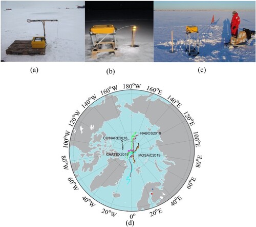
Table 1. Snow and Ice Mass Balance Apparatus (SIMBA) deployment status for various natural water environments.

Name (ID)	Location	Starting date	Thickness (m)			Sensor Interface Positions (SIPs)				Ending date
			Hi	Hs	Hf	Air/Snow	Sea Level	Snow/Ice	Ice bottom
FMI0403*	Arctic Ocean	18/08/2018	1.26	0.05	0.11	43	45	51	108	12/05/2019
FMI0505**		17/09/2018	2.11	0.03	0.47	21	21	44	126	19/09/2019
FMI0504R**		11/09/2018	2.62	0.00	0.80	23	23	63	154	24/09/2019
PRIC0903+		11/10/2018	1.74	0.14	0.24	28	35	47	122	21/04/2019
FMI0509+		08/10/2019	1.57	0.10	0.09	18	23	27	101	19/04/2020
FMI17R++		21/08/2018	1.55	0.06	0.25	42	45	58	123	28/12/2018
FMI0507++		23/08/2018	1.81	0.07	0.25	44	47	59	138	27/12/2018
FMI17	Baltic Sea	14/01/2017	0.42	0.01	−0.02	168	167	168	189	25/03/2017
FMI13		26/01/2019	0.43	0.14	0.00	90	90	90	112	01/04/2019
FMI09	Lake Orajärvi	14/12/2014	0.30	0.19	−0.03	145	146	150	163	05/02/2015
FMI0402		15/12/2016	0.31	0.08	−0.01	108	109	110	136	26/03/2017

* CHINARE2018; ** NABOS2018;+MOSAiC2019; ++ CAATEX2018 (SIPs is the initial different interface positions recorded with the SIMBA sensor number, including the air/snow interface, sea level position, snow/ice interface, and ice-bottom interface. Hi is the height of the ice, Hs is the height of the snow, and Hf is the height of the freeboard).

Figure 2. (a) Example vertical SIMBA_HT (red) and SIMBA_ET (blue) profiles observed on 14:01:12, 12 November 2018 by SIMBA FMI0504R. (b) Part of the raw SIMBA_HT time series of FMI0504R ranged from ice-freeboard to the water, from mid-January to June.

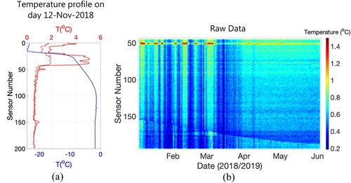
Figure 3. The part of denoised extended SIMBA_HT. Strip disturbance is removed by the streak-denoising wavelet deep neural network (SNRWDNN) model.

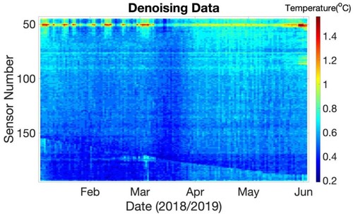
Figure 4. a) The distribution of support points for the time series collected by the buoy FMI0504R. These green points are the coordinates of support points in $P_{sub}$; b) Two boundaries of the dynamic sensor range $\mathrm{\Omega }$ and support points of $P_{sub}$. The red curve is the upper boundary, and the blue curve is the lower boundary; and c) The upper and lower boundaries of the dynamic sensor range $\mathrm{\Omega }$ and ice-bottom potential points (IBPPS).

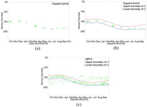
Figure 5. Identified ice-bottom (yellow dashed line) evolution by the neural network, wavelet analysis, and Kalman filtering (NWK) approach. The background represents the original SIMBA_HT time series of all sensors. The sensor numbers are converted into depth using the initial ice surface as a zero-reference level.

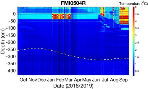
Figure 6. The neural network, wavelet analysis, and Kalman filtering (NWK) approach workflow diagram.

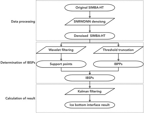
Table 2. Comparison between manual ice thickness results and NWK approach with SIMBA_HT in the Arctic Ocean.

	Stage	Mean Value (cm)		Standard Deviation (cm)		Bias (cm) (NWK)	RMSE (cm)	CORR
		Manual	NWK	Manual	NWK
FMI0403	Total	125.33	128.90	28.23	28.60	3.56	14.41	0.99
	Growth	135.55	139.52	25.22	25.00	3.96	14.41	0.99
FMI0505	Total	209.17	210.61	40.30	39.73	1.44	5.82	0.99
	Growth	182.40	184.76	20.91	21.56	2.36	6.53	0.99
	Stable	247.00	247.03	11.83	9.77	0.04	5.57	0.99
	Decay	252.66	255.04	0.94	1.14	2.37	5.71	0.98
FMI0504R	Total	208.00	206.17	31.19	30.52	−1.83	7.28	0.99
	Growth	191.86	191.19	19.63	19.38	−0.66	3.34	0.99
	Stable	244.00	242.07	5.06	4.82	−1.92	4.18	0.99
	Decay	243.00	239.06	3.21	4.01	−3.93	18.72	0.89
PRIC0903	Total	171.57	174.02	20.28	21.45	2.46	13.54	0.99
	Growth	178.00	181.71	18.30	17.73	3.71	14.90	0.99
FMI0509	Total	131.58	135.59	34.52	33.27	4.01	19.39	0.99
	Growth	146.00	149.37	27.46	26.64	3.37	13.47	0.99
FMI17R	Total	129.50	123.86	8.59	13.38	−5.64	66.85	0.95
	Growth	131.92	127.02	8.94	14.35	−4.90	62.75	0.96
FMI0507	Total	156.27	155.42	8.89	8.38	−0.85	6.39	0.96
	Growth	161.00	159.59	8.66	8.84	−1.40	2.75	0.99

Figure 7. (a) FMI0403 SIMBA_HT data and ice-bottom interface. (b) FMI0507 SIMBA_HT data and ice-bottom interface. (c) PRIC0903 SIMBA_HT data and ice-bottom surface. (d) FMI0509 SIMBA_HT data and ice interface surface. (e) FMI17R SIMBA_HT data and ice-bottom interface. (f) FMI0505 SIMBA_HT data and ice-bottom interface. (g) FMI0504R SIMBA_HT data and ice-bottom interface. The yellow dotted curve represents the ice-bottom interface.

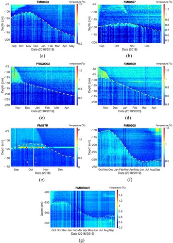
Figure 8. (a) FMI13 SIMBA_HT data and ice-bottom interface. (b) FMI17 SIMBA_HT data and ice-bottom interface. The yellow dotted curve is the ice-bottom interface.

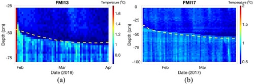
Table 3. Comparison between manual ice thickness results and the NWK approach with SIMBA_HT in the Baltic Sea.

	Stage	Mean Value (cm)		Standard Deviation (cm)		Bias (cm) (NWK)	RMSE (cm)	CORR
		Manual	NWK	Manual	NWK
FMI13	Total	56.64	55.32	4.75	4.38	−1.31	6.74	0.88
	Growth	58.09	56.38	2.59	3.51	−1.70	6.24	0.86
FMI17	Total	51.84	54.25	5.05	6.44	2.41	8.80	0.98
	Growth	53.09	56.00	3.94	4.48	2.91	9.27	0.98

Table 4. Comparison between manual ice thickness results and NWK approach with SIMBA_HT in Lake Orajärvi.

	Stage	Mean Value (cm)		Standard Deviation (cm)		Bias (cm) (NWK)	RMSE (cm)	CORR
		Manual	NWK	Manual	NWK
FMI09	Total	35.29	34.54	1.81	1.32	−0.75	2.00	0.75
	Stable	35.45	34.90	1.99	1.27	−0.54	2.02	0.76
FMI0402	Total	44.76	47.38	6.69	2.14	2.62	32.30	0.83
	Stable	49.30	48.82	3.44	2.23	−0.48	3.26	0.89

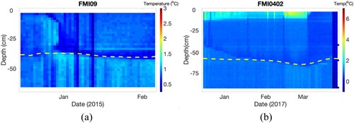
Figure 9. (a) FMI09 SIMBA_HT data and ice-bottom interface. (b) FMI0402 SIMBA_HT data and ice-bottom interface. The yellow dotted curves are the ice-bottom surface.

Data availability statement

The data that support the findings of this study are available from the corresponding author upon reasonable request.