A multi-scale path-planning method for large-scale scenes based on a framed scale-elastic grid map

Figures & data

Figure 1. Research schematic describing multi-scale path planning for large-scale scenes.

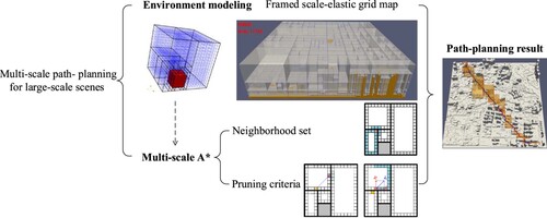
Table 1. Symbols and descriptions.

Symbol	Description
$n$	Finest-resolution grid nodes in framed multi-scale grid map
$n_{\mathrm{cur}}$	Node that currently requires neighborhood expansion
$n_{\mathrm{pre}}$	Predecessor node of $n_{\mathrm{cur}}$node
$n_{\mathrm{next}}$	Post node of $n_{\mathrm{cur}}$ node
${\mathcal{N}}_1\left(n\right)$	The set of neighborhoods formed by the spatially adjacent nodes of $n$
${\mathcal{N}}_2\left(n\right)$	The set of boundary grids of multi-scale nodes corresponding to $n$
$\mathcal{N}\left(n\right)$	The set of neighborhoods of node $n$, $\mathcal{N}\left(n\right)={\mathcal{N}}_1\left(n\right)\cup {\mathcal{N}}_2\left(n\right)$
$s$	Starting node in path-planning problems
$t$	Target node in path-planning problems
$p\left(s,t\right)$	The sequence of paths from $s$ to $t$, $p\left(s,t\right)=\{s=n_0,n_1,n_2,\dots ,n_{m-1},n_m,t=n_{m+1}$}
$d\left(n_i,n_j\right)$	Distance between nodes $n_i$ and $n_j$
$b\left(n\right)$	Multi-scale grid node corresponding to $n$

Figure 2. Illustration of 2D spatial division and identification based on the scale-elastic discrete grid structure. $L_1$ and $L_2$ denote the subdivision levels in the two directions, while $C_1$ and $C_2$ represent coordinates under different subdivision levels. The gray area in the figures depicts the range of grid identification, and corresponding numbers indicate the coordinates of the grid. (a) $L_1=0$, $L_2=1$ (b) $L_1=1$, $L_2=0$ (c) $L_1=0$, $L_2=2$ (d) $L_1=2$, $L_2=0$ (e) $L_1=1$, $L_2=1$ (f) $L_1=2$, $L_2=2$.

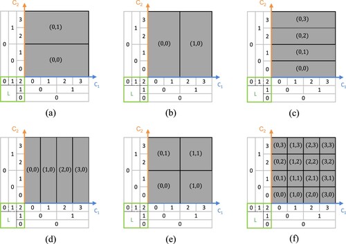
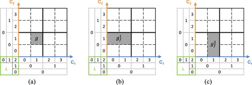
Figure 3. Parent grids in different directions. The gray grids in (b) and (c) are the parent grids of the gray grid in (a) in the $C_1$ and $C_2$ axis directions, respectively. (a) $(L_1,L_2,{\mathrm{C}}_1,{\mathrm{C}}_2)=\left(2,2,1,1\right)$ (b) $(L_1,L_2,{\mathrm{C}}_1,{\mathrm{C}}_2)=\left(1,2,0,1\right)$ (c) $(L_1,L_2,{\mathrm{C}}_1,{\mathrm{C}}_2)=\left(2,1,1,0\right)$.

Table

Algorithm 1: Grids Aggregation in the $k$-th Direction
Input: A set of grids $G=\left\{g_1,g_2,\dots ,g_m\right\}$, the direction for aggregation $k$
Output: A set of aggregated grids $G_f^k$
1: TypeA_Correspondences$=\left[\right]$
2: TypeB_Correspondences$=\left[\right]$
3: AggregatedGrids$=\left[\right]$
4: for each grid $g_i$in G do
5:    // Calculate the parent grid of $g_i$ in the $k$-th direction
6:    $g_{\mathrm{if}}^k=$Calculate parent grid ($g_i$, $k$)
7:    TypeA_Correspondences.append (($g_{\mathrm{if}}^k$, $g_i$))
8: end for
9: // Merge type A correspondences with the same parent grid into type B correspondences
10: for each correspondence ($g_f^k,g$) in TypeA_Correspondences do
11:    Related_Correspondences = Filter TypeA_Correspondences with parent grid $g_f^k$
12:    if the size of Related_Correspondences > 1 then
13:       Child_Grids = Extract child grids from Related_Correspondences
14:       TypeB_Correspondences.append (($g_f^k$, Child_Grids))
15:       for each correspondence in Related_Correspondences do
16:           TypeA_Correspondences.remove (correspondence)
17:       end for
18:    end if
19: end for
20: // Generate aggregated grids
21: for each correspondence ($g_f^k$, $g$) in TypeA_Correspondences do
22:    AggregatedGrids.append ($g$)
23: end for
24: for each correspondence ($g_f^k$, Child_Grids) do
25:    AggregatedGrids.append $g_{\mathrm{if}}^k)$
26: end for
27: return AggregatedGrids

Figure 4. Illustration of grid-set aggregation.

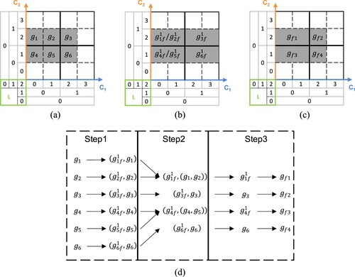
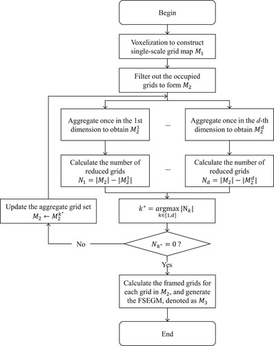
Figure 5. Flow chart for construction of framed scale-elastic grid map (FSEGM).

Table

Algorithm 2: Generate Framed Scale-elastic Gird Map
Input: A single-scale grid map $M_1$ at the finest resolution level
Output: Framed scale-elastic grid map $M_3$
1: $M_2=$Filter out the occupied grids from $M_1$
2: repeat
3:    for $k$ = 1 to $d$ do
4:       $M_2^k=$AggregateGrids ($M_2$, $k$)
5:      $N_k=\left|M_2\right|-\left|M_2^k\right|$
6:    end for
7:   $k^{\ast }=\underset{k\in \left[1,d\right]}{\mathrm{argmax}}\left(N_k\right)$
8: until $N_{k^{\ast }}=0$
9: $M_2=M_2^{k^{\ast }}$
10: $M_3=\left[\right]$
11: for each grid $g$ in $M_2$ do
12:    FramedGrids$=$Cal the framed grids of $g$
13:    $M_3$.append (FramedGrids)
14: end for
15: return $M_3$

Figure 6. Various grid maps of the same environment. The blue and red grids represent barrier-free and barrier areas, respectively. (a) example scenario (b) single-scale grid map (c) framed-octree grid map (d) FSEGM.

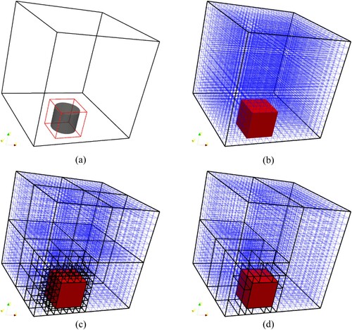
Figure 7. Different types of neighborhoods in a 2D environment.

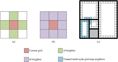
Figure 8. Illustration of neighborhood range pruning in a 2D environment. (a) Range of $\mathcal{N}\left(n_{\mathrm{cur}}\right)$ without pruning, (b) Range of nodes to be explored ($S_1$) after neighborhood range pruning.

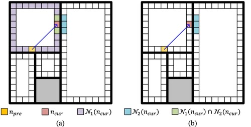
Figure 9. Illustration of exploration-direction pruning in a 2D environment. (a) Range of ${\mathcal{N}}_2\left(n_{\mathrm{cur}}\right)$ without pruning, (b) Range of ${\mathcal{N}}_2\left(n_{\mathrm{cur}}\right)$ after directional pruning.

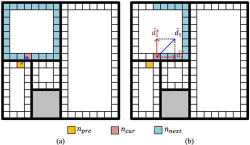
Figure 10. Illustration of the proof of the optimality criterion for exploration-direction pruning in a 2D environment.

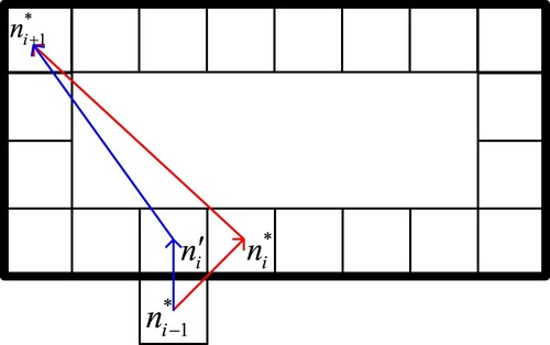
Figure 11. Scene-vector data and voxelized scene models at different levels. The map sizes of (b) – (e) are $32\times 32\times 8$, $64\times 64\times 16$, $128\times 128\times 32$, $256\times 256\times 64$, $512\times 512\times 128$, respectively. (a) Local city scenes of Zhengzhou (b) ${\mathrm{V}}_1$ (c) ${\mathrm{V}}_2$ (d) ${\mathrm{V}}_3$ (e) ${\mathrm{V}}_4$ (e) ${\mathrm{V}}_5$.

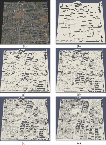
Figure 12. Illustration of different types of grid maps corresponding to ${\mathrm{V}}_3$: (a) SGM, (b) FOGM, and (c) FSEGM.

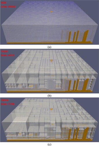
Table 2. Number of grids and border grids required to build each type of grid map for maps of different sizes.

	SGM	FOGM		FSEGM		Percentage Decrease
		$\mathrm{grid}$	$\mathrm{border}\mathrm{grid}$	$\mathrm{grid}$	$\mathrm{border}\mathrm{grid}$	$\mathrm{grid}$	$\mathrm{border}\mathrm{grid}$
${\mathrm{V}}_1$	4974	1684	4798	652	4630	61.3%	3.5%
${\mathrm{V}}_2$	46652	8544	39724	2707	36748	68.3%	7.5%
${\mathrm{V}}_3$	409265	44313	279025	11788	247729	73.4%	11.2%
${\mathrm{V}}_4$	3447814	213268	1752006	51481	1499686	75.9%	14.4%
${\mathrm{V}}_5$	28389549	998689	10206541	214309	8420469	78.5%	17.5%

Figure 13. Number of (a) grids and (b) border grids required to build FOGM and FSEGM for models ${\mathrm{V}}_1\text{–}{\mathrm{V}}_5$.

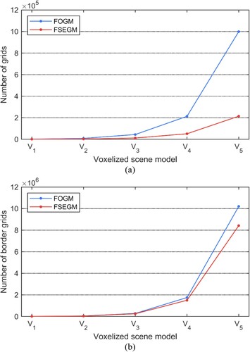
Figure 14. Time required to build SGM, FOGM and FSEGM for models ${\mathrm{V}}_1\text{–}{\mathrm{V}}_5$.

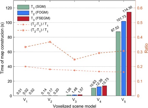
Figure 15. Illustration of path planning results (left column: side view; right column: top view) for (a)(b) SGM + A*, (c)(d) FOGM + A*, (e)(f) FOGM + Multi-scale A*, (g)(h) FSEGM + A*, and (i)(j) FSEGM + Multi-scale A*.

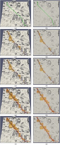
Figure 16. Statistical results of path planning indicators. $c_1$: number of maintained nodes; $c_2$: number of searched nodes; $c_3$: number of planned path nodes; $c_4$: length of planned path; $c_5$: path-planning time. The units of $c_4$ and $c_5$ are meters and milliseconds, respectively.

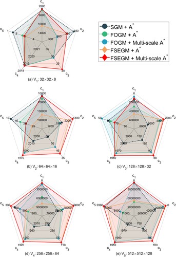
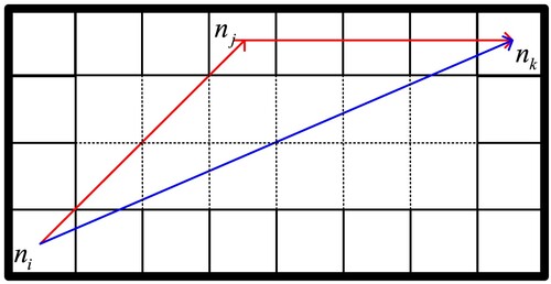
Figure 17. Illustration of the planning length gap. Thick solid line: Node in FMGM (FOGM or FSEGM); Thin solid line: border grids for the node; Dashed line: Aggregated single-scale grid in the node. The red line indicates the optimal path from $n_i$ to $n_k$ planned in SGM. The blue line indicates the optimal path from $n_i$ to $n_k$ planned in FMGM.

Data availability statement

The data that support the findings of this study are available at https://www.scidb.cn/anonymous/N2JJUnZh.