Realistic potential increases in carbon storage via timber rotation extensions: an analysis of the Pacific Northwest

Figures & data

Figure 1. The study area (Highlighted by a red square) comprises Washington and Oregon.

Figure 2. The modeled age at which stands are expected to reach the culmination of mean annual increment (CMAI) is gridded at a 0.2 × 0.2° latitude–longitude Resolution. This age varies widely across the Pacific Northwest. While small-scale variability likely represents noise, larger-scale patterns reveal regional characteristics. Please note that the color scale saturates at 30 and 100 years.

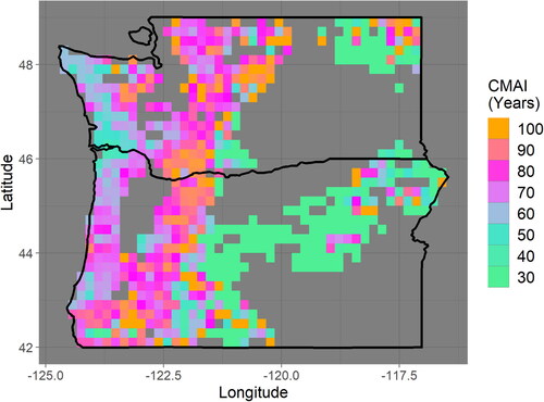
Figure 3. Maps of the ages and aboveground live biomass carbon densities beyond optimal CMAI-constrained medians reveal large areas containing negative values, which indicate that the median age (panel (a)) and median carbon density (panel (b)) are less than what would be expected under a harvest schedule informed by CMAI. Approximately 9% of forested area grid cells contain such a carbon density deficit at 90% confidence, indicated by stippling. In western Washington and northwestern Oregon, these deficits are generally greater than 100 MTCO₂ ha⁻¹. The color scale saturates at a magnitude of 30 (panel (a)) and 300 (panel (b)).

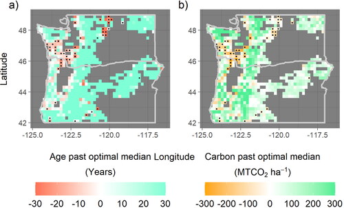
Figure 4. Data is displayed in the manner of Figure 2, panel (b), but optimal rotation length is defined by both CMAI and diameter threshold. The percent of grid cells in a carbon deficit at 90% confidence declines from approximately 9% to approximately 7%, with a particularly large loss of statistically significant deficit in western Washington. Some areas in western Washington completely lose a carbon deficit when diameter limitations are accounted for, while other simply decline in carbon deficit magnitude from nearly 200 to closer to 100 MTCO₂ ha⁻¹, with much of this remaining carbon deficit becoming statistically insignificant because of large uncertainties. As in Figure 2 panel (b), the color scale saturates at a magnitude of 300.

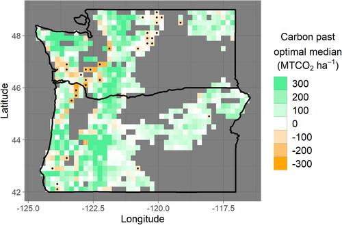
Figure 5. Eastern Washington contains large areas of forests owned by corporate entities and timber investment management operations (TIMOs). the total area in each 0.2 × 0.2° latitude–longitude grid cell at this latitude is approximately 35,000 ha.

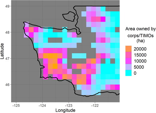
Figure A1. (a) FIA sites with nonzero live tree biomass are projected onto the first two PCA axes, which together account for 8.7% of variability across 10,305 sites. Species associated with the most variability are (clockwise from upper left) WR (western redcedar), WH (western hemlock), PSF (Pacific silver fir), MH (Mountain hemlock), SF (subalpine fir), ES (Engelmann spruce), LP (lodgepole pine), PP (ponderosa pine), PM (Pacific madrone), and DF (Douglas fir). (b) In coastal areas, most forests are associated with the presence of Douglas fir, western hemlock, and/or western redcedar.

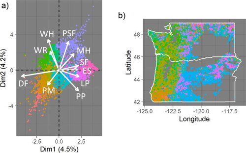
Figure A2. When fitted growth parameters for each site are used to reproduce the aboveground live tree carbon of the corresponding site, the aggregated residuals are centered at zero, slightly skewed, and highly peaked. While the residuals for each parameter fitting for each individual site are assumed either normal or skew-normal (i.e. having a smaller peak than is seen here), a greater number of fittings that produce lower variance and a smaller number of fittings that produce a higher variance would produce this high peak when all residuals are aggregated. Fittings all allow for skew in the residuals (a characteristic that may be preserved in residual aggregation if skew occurs more often in one direction) and assume unbiasedness of the model (a characteristic that would be preserved during residual aggregation), so these characteristics of the aggregated residuals distribution are also consistent with the prior assumptions used in model fitting. The width of the bins in this histogram is 10 MT CO₂ ha⁻¹. A white vertical line overlaying the histogram designates zero.

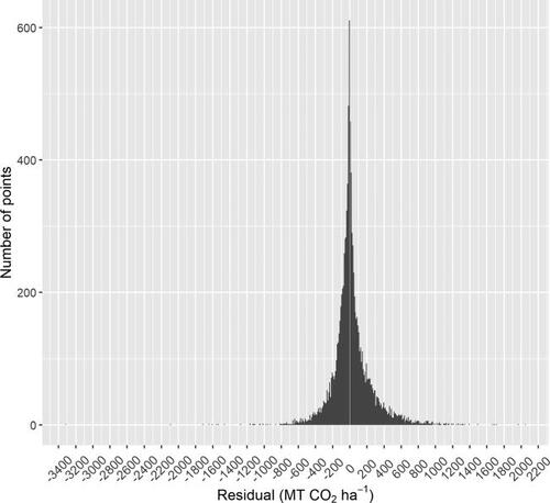
Figure A3. Modeled versus observed aboveground live tree carbon approximately follow the 1:1 line (denoted in white).

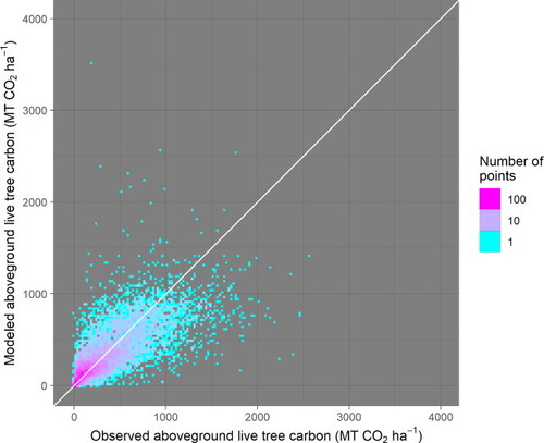
Figure A4. Aggregated residuals are unbiased by stand age. They do, however, display an increased variance with increased stand age, and this phenomenon is accounted for in the prior assumptions used in model fitting (Text A1.3). Please note that one datapoint is eliminated from this figure because of a reported stand age of 10,000 years.

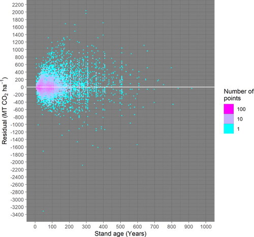
Figure A5. The residuals do not show a correlation with modeled carbon. The variance of residuals does increase with modeled carbon, a phenomenon related to increasing variance with stand age, which is accounted for in the model fitting (Text A1–A4). Because all values are bounded at zero (i.e. carbon stocks cannot be negative), residuals are bounded at the −1:1 line.

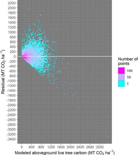
Figure A6. The geographic distribution of residuals for all sites with recorded live trees shows no clear geographical biases. The magnitude of residuals, however, does vary with geography, but this phenomenon can be explained by the variation of average stand age with geography (Figure A7). the relationship between residual magnitude and stand age is accounted for in the model fitting (Text A1–A4).

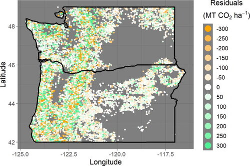
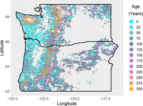
Figure A7. the geographical differences in stand age can explain the geographical differences in residual magnitude seen in Figure A6.

Data availability statement

All tree level, plot level, and condition level Forest Inventory and Analysis (FIA) data used in this analysis can be found at the FIA DataMart at https://apps.fs.usda.gov/fia/datamart/datamart.html courtesy of the United States Forest Service (USFS).

The forest ownership data used in this analysis can be found at the USFS Research Data Archive at https://www.fs.usda.gov/rds/archive/Catalog/RDS-2020-0044.