Distributed control for bi-connectivity of multi-robot network

Figures & data

Figure 1. Preservation and improvement of network bi-connectedness.

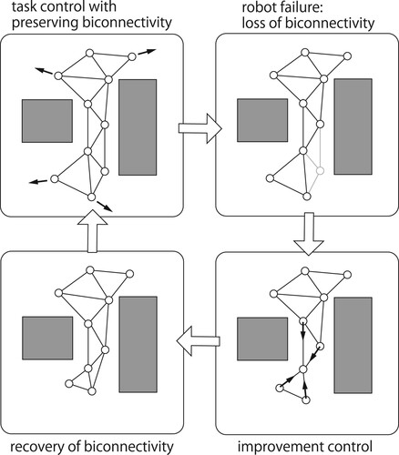
Figure 2. Illustrated description of link weight functions Equations (2(2) $a_{ij}={\gamma }^a\left({\mathrm{d}\mathrm{i}\mathrm{s}\mathrm{t}}_{ij}\right)\prod _{k\in {\mathcal{O}}_{ij}}{\gamma }^b\left({\mathrm{d}\mathrm{i}\mathrm{s}\mathrm{t}}_{ijk}\right),$(2) )–(4(4) ${\gamma }^b\left({\mathrm{d}\mathrm{i}\mathrm{s}\mathrm{t}}_{ijk}\right)={(1+\exp (-{\alpha }_b(\frac{{\mathrm{d}\mathrm{i}\mathrm{s}\mathrm{t}}_{ijk}}{d_{max}}-{\text{β}}_b)))}^{-1},$(4) ). (a) Definition of ${\mathrm{d}\mathrm{i}\mathrm{s}\mathrm{t}}_{ij}$ and ${\mathrm{d}\mathrm{i}\mathrm{s}\mathrm{t}}_{ijk}$. (b) ${\gamma }^a$ with respect to ${\mathrm{d}\mathrm{i}\mathrm{s}\mathrm{t}}_{ij}$ and (c) ${\gamma }^b$ with respect to ${\mathrm{d}\mathrm{i}\mathrm{s}\mathrm{t}}_{ijk}$.

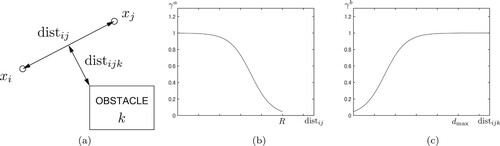
Figure 3. Numerical demonstration of sufficient condition Equation (11(11) ${\hat{\lambda }}^{\left(i\right)}>\frac{N}{5N-9},$(11) ). (a) ${\hat{\lambda }}^{\left(i\right)}$ v.s. # of connected component in ${\mathcal{G}}_{-i}$ and (b) Numerical maximum of ${\hat{\lambda }}^{\left(i\right)}$.

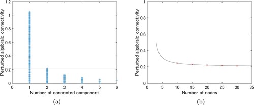
Figure 4. Artificial potential function $V\left({\tilde{\lambda }}^{\left(i\right)}\right)$.

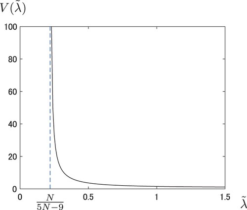
Figure 5. Robots on boundary of convex hull $\mathcal{C}$ move into $\mathcal{C}$.

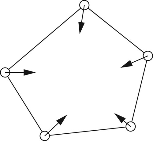
Figure 6. Difficult situation to resume bi-connectivity while keeping other non-articulation nodes.

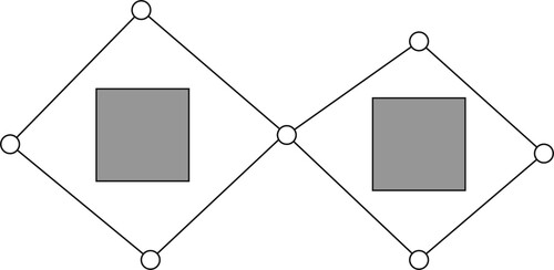
Figure 7. Snapshots of simulation 1. (a) Initial configuration (t = 0). (b) Node 20 is restored at t = 1.9 and (c) Final configuration at t = 10.

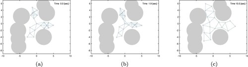
Figure 8. Perturbed algebraic connectivity ${\tilde{\lambda }}^{\left(20\right)}$ versus time t.

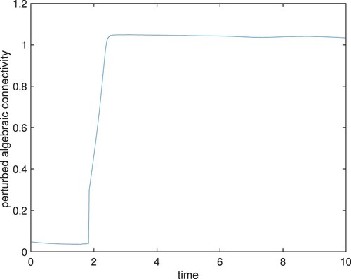
Figure 9. Snapshots of simulation 2. (a) Initial configuration (t = 0). (b) t = 20 and (c) t = 80.

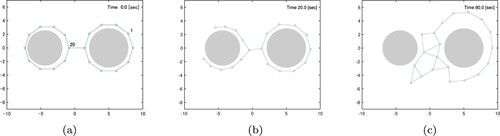
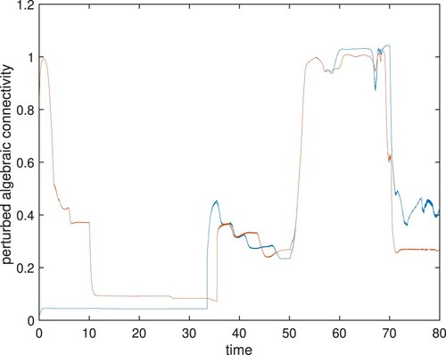
Figure 10. Perturbed algebraic connectivities ${\tilde{\lambda }}^{\left(20\right)}$ (blue line) and ${\tilde{\lambda }}^{\left(1\right)}$ (red line) versus time t. Node 1 is initially non-articulation but becomes an articulation node to restore the bi-connectivity of the entire network.