Receptor occupancy assessment and interpretation in terms of quantitative systems pharmacology: nivolumab case study

Figures & data

Figure 1. Scheme of the PK-RO model for mAbs targeting PD-1 receptor. The PK module describes pharmacokinetics utilizing a generic two-compartmental model with zero-order intravenous (IV) infusion. The PD-1 module describes the dynamics of PD-1 receptors (synthesis, degradation, and internalization) as well as receptor interactions with mAb at the cellular surface.

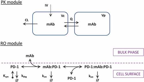
Figure 2. Observed and model predicted trough PD-1 occupancy depending on nivolumab dose level. The trough receptor occupancy in peripheral blood was assessed at day 56 of treatment at a dose of 0.1 to 10 mg/kg Q2W. Red symbols represent the clinical data (mean ± SD); blue symbols correspond to the model simulations (median with 95% CI).

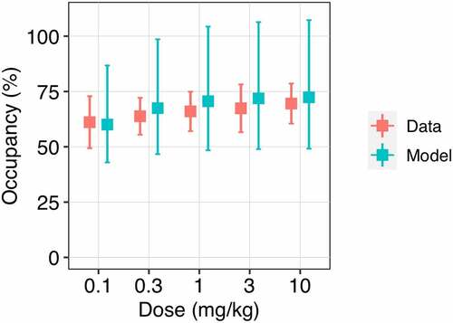
Figure 3. Observed and model predicted profiles of PD-1 occupancy after multiple administration of nivolumab 10 mg/kg. (a) Equation 3(3) $RO\mathrm{\%}=100\cdot \left(\frac{R_{bound}}{R_{total}^{predose}}\right)=100\cdot \left(\frac{\left[mAb\cdot R\right]+\left[R\cdot mAb\cdot R\right]}{{\left[R\right]}_{baseline}}\right)$(3) was used to generate the RO profile with receptor normalization to the baseline level. (b) Equation 4(4) $RO\mathrm{\%}=100\cdot \left(\frac{R_{bound}}{R_{total}}\right)=100\cdot \left(\frac{\left[mAb\cdot R\right]+\left[R\cdot mAb\cdot R\right]}{\left[R\right]+\left[mAb\cdot R\right]+2\cdot \left[R\cdot mAb\cdot R\right]}\right)$(4) was used to generate the RO profile with receptor normalization at each time point. Symbols represent the clinical data (mean ± SD); solid lines correspond to the model simulations (median with 95% CI).

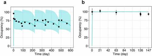
Figure 4. Comparison of PD-1 occupancy profiles generated utilizing different strategies of RO assessment. (a) Equation 1(1) $RO\mathrm{\%}=100\cdot \left(1-\frac{R_{free}}{R_{free}^{predose}}\right)=100\cdot \left(1-\frac{\left[R\right]}{{\left[R\right]}_{baseline}}\right)$(1) versus equation 2(2) $RO\mathrm{\%}=100\cdot \left(1-\frac{R_{free}}{R_{total}}\right)=100\cdot \left(1-\frac{\left[R\right]}{\left[R\right]+\left[mAb\cdot R\right]+2\cdot \left[R\cdot mAb\cdot R\right]}\right)$(2) – free receptor measurements with normalization to baseline and at each time point, respectively; (b) equation 3(3) $RO\mathrm{\%}=100\cdot \left(\frac{R_{bound}}{R_{total}^{predose}}\right)=100\cdot \left(\frac{\left[mAb\cdot R\right]+\left[R\cdot mAb\cdot R\right]}{{\left[R\right]}_{baseline}}\right)$(3) versus equation 4(4) $RO\mathrm{\%}=100\cdot \left(\frac{R_{bound}}{R_{total}}\right)=100\cdot \left(\frac{\left[mAb\cdot R\right]+\left[R\cdot mAb\cdot R\right]}{\left[R\right]+\left[mAb\cdot R\right]+2\cdot \left[R\cdot mAb\cdot R\right]}\right)$(4) – bound receptor measurements with normalization to baseline and at each time point, respectively; (c) equation 1(1) $RO\mathrm{\%}=100\cdot \left(1-\frac{R_{free}}{R_{free}^{predose}}\right)=100\cdot \left(1-\frac{\left[R\right]}{{\left[R\right]}_{baseline}}\right)$(1) and equation 3(3) $RO\mathrm{\%}=100\cdot \left(\frac{R_{bound}}{R_{total}^{predose}}\right)=100\cdot \left(\frac{\left[mAb\cdot R\right]+\left[R\cdot mAb\cdot R\right]}{{\left[R\right]}_{baseline}}\right)$(3) – free and bound receptor measurements with normalization to baseline, respectively; (d) equation 2(2) $RO\mathrm{\%}=100\cdot \left(1-\frac{R_{free}}{R_{total}}\right)=100\cdot \left(1-\frac{\left[R\right]}{\left[R\right]+\left[mAb\cdot R\right]+2\cdot \left[R\cdot mAb\cdot R\right]}\right)$(2) and equation 4(4) $RO\mathrm{\%}=100\cdot \left(\frac{R_{bound}}{R_{total}}\right)=100\cdot \left(\frac{\left[mAb\cdot R\right]+\left[R\cdot mAb\cdot R\right]}{\left[R\right]+\left[mAb\cdot R\right]+2\cdot \left[R\cdot mAb\cdot R\right]}\right)$(4) – free and bound receptor measurements with normalization at each time point, respectively. The simulations were conducted for a single infusion of nivolumab at a flat dose of 240 mg. Solid lines correspond to the model simulations (median with 95% CI).

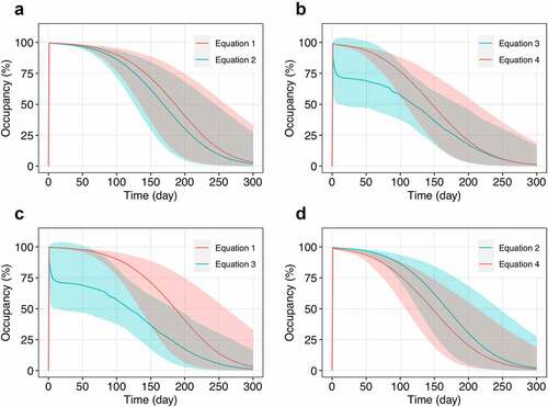
Figure 5. Different formats of receptor occupancy assays and equations utilized for occupancy calculation. (a) Scheme reflecting the links between flow cytometry strategies for RO assessment and corresponding equations for RO calculation. (b) An example of PD-1 occupancy calculations based on raw MFI data, which results in different occupancy values. The initial table contains MFI values (subtracting background signal) corresponding to the drug bound to receptor and to the total receptor, respectively. The upper table and graph represent RO values calculated with equation 3(3) $RO\mathrm{\%}=100\cdot \left(\frac{R_{bound}}{R_{total}^{predose}}\right)=100\cdot \left(\frac{\left[mAb\cdot R\right]+\left[R\cdot mAb\cdot R\right]}{{\left[R\right]}_{baseline}}\right)$(3) , whereas the lower table and graph represent RO values calculated with equation 4(4) $RO\mathrm{\%}=100\cdot \left(\frac{R_{bound}}{R_{total}}\right)=100\cdot \left(\frac{\left[mAb\cdot R\right]+\left[R\cdot mAb\cdot R\right]}{\left[R\right]+\left[mAb\cdot R\right]+2\cdot \left[R\cdot mAb\cdot R\right]}\right)$(4) . The results diverge due to different normalization during RO calculations.

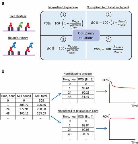
Table 1. Overview of the model parameters and their origin.

Parameter [Units]	Estimate	Inter-individual variability ω^Citation2	Source
Pharmacokinetic module
$Vc$ [L]	3.63	0.123	23
$CL$ [L/h]	0.0094	0.123	23
$Vp$ [L]	2.78	0.258	23
$Q$ [L/h]	0.0321	–	23
$V{c}_{BW}$ [unitless]	0.597	–	23
$C{L}_{BW}$ [unitless]	0.566	–	23
PD-1 receptor module
$K_{syn}$ [item/h]	$k_{deg}\cdot PD{1}_{baseline}$	–	–
$k_{deg}$ [1/h]	0.01402	0.645	27
$PD{1}_{baseline}^{CD4}$ [item]	2213	0.272	18
$PD{1}_{baseline}^{CD8}$ [item]	2639	0.258	18
$k_{int}$ [1/h]	$k_{deg}/Expression$	–	–
$Expression$ [unitless]	0.752	0.218	16, 18
$k_{off}$ [1/h]	2.7648	–	14
$K{d}_{3D}$ [nM]	3.06	–	14
$S{A}_{cell}$ [μm^Citation2]	152	–	28

$Vc$, central compartment; $CL$, clearance; $Vp$, peripheral compartments; $Q$, inter-compartmental clearance; $V{c}_{BW}$ and $C{L}_{BW}$, the body weight covariates for central compartment and clearance; $K_{syn}$, PD-1 synthesis rate; $k_{deg}$, rate constant of PD-1 degradation; $PD{1}_{baseline}^{CD4}$ and $PD{1}_{baseline}^{CD8}$, baseline level of PD-1 at the surface of CD4 and CD8 T cells, respectively; $k_{int}$, rate constant of bound PD-1 internalization; $Expression$, fold change in PD-1 expression during treatment; $k_{off}$, dissociation rate constant of nivolumab:PD-1 complex; $K{d}_{3D},$ dissociation constant of nivolumab:PD-1 complex in the solution; $S{A}_{cell}$, surface area of the T cell.

Liang M, Schwickart M, Schneider AK, Vainshtein I, Del Nagro C, Standifer N, Roskos LK. Receptor occupancy assessment by flow cytometry as a pharmacodynamic biomarker in biopharmaceutical development. Cytometry B Clin Cytom. 2016;90(2):117–27. doi:10.1002/CYTO.B.21259.

 PubMed Web of Science ®Google Scholar