Selection of target-binding proteins from the information of weakly enriched phage display libraries by deep sequencing and machine learning

Figures & data

Figure 1. Three-dimensional structure of the entire sequence of 2u2f. The two randomized loops are in red.

Scaffold protein structure where the randomized region is colored red.

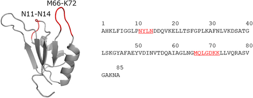
Figure 2. Workflow of biopanning. At each round, 1) target-bound phages were selected, 2) E. coli was infected with selected phages, and 3) phages were amplified in E. coli. Sub-libraries are surrounded by colored ellipses.

The workflow of four rounds selecting target-bound phages from initial phages and amplified phages.

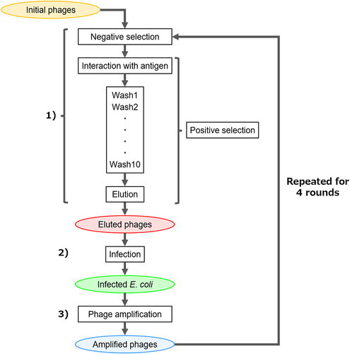
Figure 3. Distribution of unique sequences in each sub-library. The frequency of unique sequences is shown for single reads in gray, 2–10 reads in blue, 11–100 reads in green, 101–200 reads in yellow, 201–1000 reads in brown, and >1000 reads in red.

The frequency of unique sequences in sub-libraries which are phage pools or E. coli collected during biopanning.

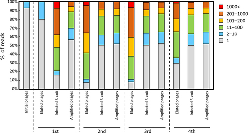
Figure 4. Amino acid frequencies and rank distribution of the sequences predicted by machine learning. (a) Amino acid frequencies of top 10,000 sequences predicted by machine learning, visualized by WebLogo.⁴¹ (b) Amino acid frequencies of clustered sequences. (c) Rank distribution of each cluster. Black arrows indicate clusters containing the top 1,000 sequences.

The top 10,000 sequences predicted by machine learning were clustered into nine distinct sequence patterns. Each cluster had a distribution with different averages.

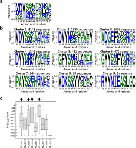
Figure 5. Binding function of wild-type 2u2f and obtained 2u2f variants. (a) Enzyme-linked immunosorbent assay of the candidate 2u2f variants after purification on galectin-3 (Gal), NeutrAvidin (NAV), or blocking buffer (Skim). (b) EC₅₀ values of wild-type 2u2f and four functional variants with affinity to galectin-3. The plots show the absorbance of galectin-3 minus that of NAV. The EC₅₀ values were determined by using Hill equation.

In an enzyme-linked immunosorbent assay of the candidate 2u2f variants, four 2u2f variants are specifically bound to the target molecule with the EC 50 values of 93 nanomolar, 80 nanomolar, 277 nanomolar, and 201 nanomolar.

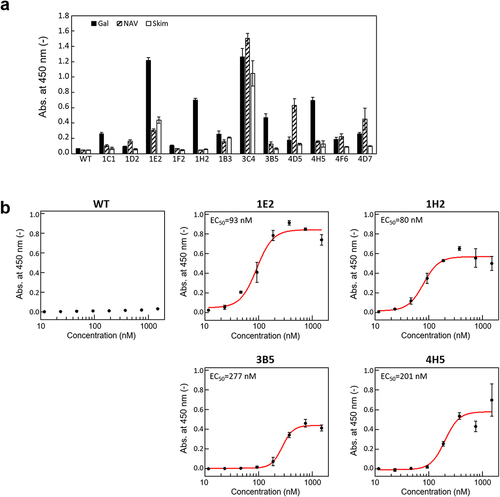
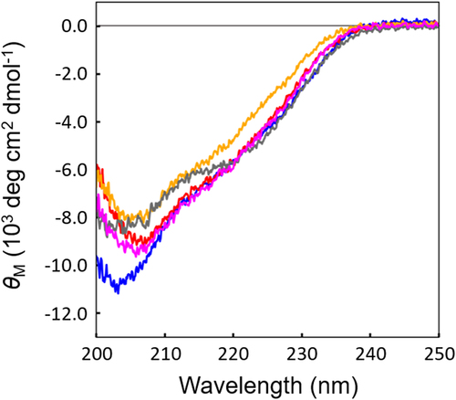
Figure 6. CD spectra of the functional 2u2f variants. Wild-type 2u2f is shown in blue, 1E2 in Orange, 1H2 in red, 3B5 in gray, and 4H5 in magenta.

Circular dichroism spectra showing that the secondary structures of four prospective variants were similar to those of wild-type 2u2f.

Crooks GE, Hon G, Chandonia JM, Brenner SE. WebLogo: a sequence logo generator. Genome Res. 2004;14(6):1188–90. doi:10.1101/gr.849004.

 PubMed Web of Science ®Google Scholar