Crowd model calibration at strategic, tactical, and operational levels: Full-spectrum sensitivity analyses show bottleneck parameters are most critical, followed by exit-choice-changing parameters

Figures & data

Figure 1. The overall structure of the computational simulation modelling tool employed in this work. Illustrating various behavioural layers of the model, the nature (or type) of the model at each layer and the parameters involved in each layer.

Table 1. The list of the parameters of the simulation model, their descriptions, and the calibrated (or suggested) values. The asterisk indicates the parameters whose values have been calibrated empirically and are the subject of the sensitivity analyses in this work.

Parameter	Description	Calibrated value
λ	Parameter related to the mean and variance of the reaction times. Default value is positive. Greater values mean smaller reaction times as well as less variability in reaction times across simulated occupants.	1.523*
ν	Parameter related to the reaction times. Default value is positive. Not subject of the sensitivity analyses.	2.511
μ	Parameter that determines the effect of distance to nearest exit (at the onset of evacuation) on reaction time. Default value is negative. Greater absolute values mean that the further the agent is to exits, the longer it takes for it to initiate movement.	−0.305*
θ	Parameter related to the room sequence choice reflecting the effect of distance to the final gates on room sequence choice. Default value is positive. Greater values mean that the agent is more likely to choose the room sequence that offers the minimum distance to a final exit.	0.500
${\beta }_{\mathit{DIST}}$	Parameter related to the exit choice reflecting the effect of the distance to exits on exit choice. Default value is negative. Greater absolute values mean that the agent is more likely to choose the nearest distance.	−0.278*
${\beta }_{\mathit{CONG}}$	Parameter related to the exit choice reflecting the effect of the queue size (congestion) on exit choice. Default value is negative. Greater absolute values mean that the agent is more likely to choose the least congested exit.	−0.158*
${\beta }_{\mathit{FLTOVIS}}$	Parameter related to the exit choice reflecting the effect of the flow size on exit choice (for the exits that are visible). Default value is negative. Greater absolute values mean that the agent is more likely to avoid the visible exits to which heavy flows are moving.	−0.042*
${\beta }_{\mathit{FLTOINVIS}}$	Parameter related to the exit choice reflecting the effect of the flow size on exit choice (for the exits that are invisible). Default value is positive. Greater values mean that the agent is more likely to follow the invisible exits to which heavy flows are moving.	0.013*
${\beta }_{\mathit{VIS}}$	Parameter related to the exit choice reflecting the effect of the exit visibility on exit choice. Default value is positive. Greater values mean that the agent is more likely to choose the exits that are visible.	0.802*
${\alpha }_{\mathit{Inertia}}$	Parameter related to the exit-choice-changing behavior reflecting the tendency of the agent to maintain the initial choice of exit. Default value is negative. Greater absolute values mean that the agent is more likely to choose to not to change the previous choice of exit when given the opportunity to revise that decision.	−7.234*
${\alpha }_{\mathit{CongRatio}}$	Parameter related to the exit-choice-changing behavior reflecting the relative queue size at the chosen exit compared to that of the least congested exit in that room. Default value is positive. Greater values mean that the agent is more likely to choose to change the previous choice of exit when the queue at that exit is relatively large.	3.119*
${\alpha }_{\mathit{SocInf}}$	Parameter related to the exit-choice-changing behavior reflecting the social (or peer) influence. Default value is positive. Greater values mean that the agent is more likely to choose to change the previous choice of exit when other agents have made the same change during earlier moments.	0.577*
${\alpha }_{\mathit{Vis}}$	Parameter related to the exit-choice-changing behavior reflecting the exit visibility effect. Default value is positive. Greater values mean that the agent is more likely to choose to change the previous choice of exit when a less congested exit in that room is within its visual field.	1.876*
ω	Penalty weight for the weighted shortest path algorithm. Greater values mean that the agent will avoid the areas occupied by other agents and takes longer detours to reach the chosen exit.	4500
τ	Relaxation parameter of the social-force model. Default value is positive. Greater values mean that the driving force is weaker, and that the bottleneck flow rate is slower.	0.120*
κ	Friction force parameter of the social force model. Default is positive. Greater values mean that the friction force between the agent and other agents or walls that are in physical contact with the agent is greater, and that the bottleneck flow rate is slower.	5500*
A	Social force parameter related to interindividual and wall forces when there is no physical contact. Default is positive. Greater values mean that the agent perceives greater repulsion forces from other agents or the walls when there is no contact with them.	2000
B	Social force parameter related to interindividual and wall forces. Default is positive. Greater values mean that the agent perceives smaller repulsion forces from other agents or the walls when there is no contact with them.	0.080
k	Social force parameter related to interindividual and wall forces. It determines the obstruction effects in cases of physical interactions	120000

Table 2. The list of the variables and their description in the simulation model.

Variable	Description
Min_Exit_DISTi	Euclidian distance of agent i to the nearest exit in the current room at the onset of the evacuation
Room_Seq_DISTir	The distance from the position of agent i, to the nearest final gate through room sequence r, at the onset of the evacuation
DISTie	The Euclidian distance from the position of agent i, to exit e
CONGie	The queue size (congestion) at exit e observed by agent i
FLOWie	The flow size moving to exit e observed by agent i
VISie	The visibility status of exit e according to agent i, equals 1 if visible and 0 otherwise
Min_CONGi	The queue size at the least congested exit in the current room of agent i
CONGie*	The queue size at the currently chosen exit e^* by agent i
Visi	The congestion-visibility status for agent i, equals 1 if there is a visible AND less congested exit available at the current room for agent i, and 0 otherwise
SocInfi	The social influence on exit-choice change for agent i. The number of other agents changing their decisions from e* to another exit within the last t=2 seconds of the simulated time
mi	The body mass of agent i
$\overrightarrow{r}\mathit{i}$	The body ratio of agent i
$v_i^d$	The desired velocity of agent i
${\vec{e}}_{\mathit{i}}^{\mathit{d}}$	The unit vector of desired direction for agent i
dij	The Euclidian distance between agents i and j
diw	The Euclidian distance between agent i and wall w

Figure 2. Still images from the data extraction process of a sample of scenarios in Experiment I. Subfigure (a) shows an exit-choice observation extraction example and subfigure (b) shows an example of data extraction for exit choice adaptation. Both figures only illustrate the moment of observation extraction. At such moments, the set of information regarding the subject’s decision is recorded including the choice, choice set and attribute levels of the alternatives.

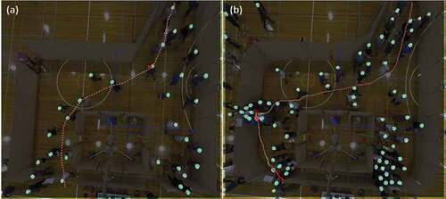
Figure 3. Still images from the data extraction process of a sample of scenarios in Experiment II. Subfigure (a) shows an exit-choice observation extraction example and subfigure (b) shows an example of data extraction for exit choice adaptation. Both figures only illustrate the moment of observation extraction. At such moments, the set of information regarding the subject’s decision is recorded including the choice, choice set and attribute levels of the alternatives.

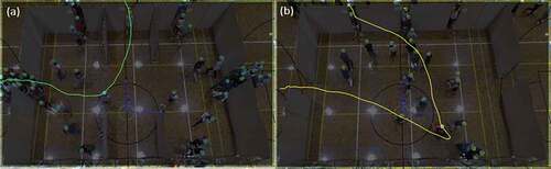
Figure 4. Still images from the data extraction process of a sample of scenarios in Experiment III. Subfigure (a) shows a reaction-time observation extraction example and subfigure (b) shows an example of data extraction for exit choice adaptation.

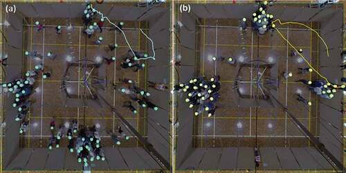
Figure 5. Still image from the setup of the Experiment IV, the bottleneck experiment.

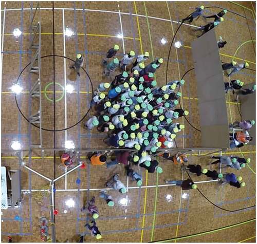
Table 3. The list of experiments whose observations were used for the calibration of the numerical simulation model used in this study.

Experiment No.	Year	No. of participants	No. of scenarios	Relevance to calibration
I	2015	142	29	Exit choice Exit choice change
II	2017	114	24	Exit choice Exit choice change
III	2017	146	24	Reaction time Exit choice change
IV	2017	114	21	Social force (at bottlenecks)

Figure 6. A visualisation of the parameter calibration process for the key parameters of the social force layer of our simulation model based on observations of the total evacuation time obtained from Experiment IV. Plots (1)-(6) are respectively related to the bottleneck scenarios with exit width 60cm-120cm. Regions of each graph with brighter colour represent the parameter combinations that produced the least amount of simulation error for that scenario. Note that, the scale of the plot legend does not need to match across different exit widths, because for each exit width, the best parameter combinations are chosen independent of the other exit widths. The chosen parameter combination is one that resides at the intersect of the ‘best parameter combinations list’ for all seven different widths.

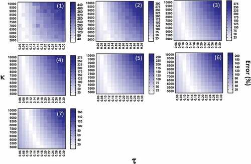
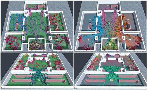
Figure 7. Still images from the visualisation of the numerical calculation processes for setups 1–4. A video visualisation of the simulation process associated with each setup can be viewed and/or downloaded from the links below. Note that the videos are corresponding to simulation at default/calibrated parameters, and not any deviation from the calibrated values.

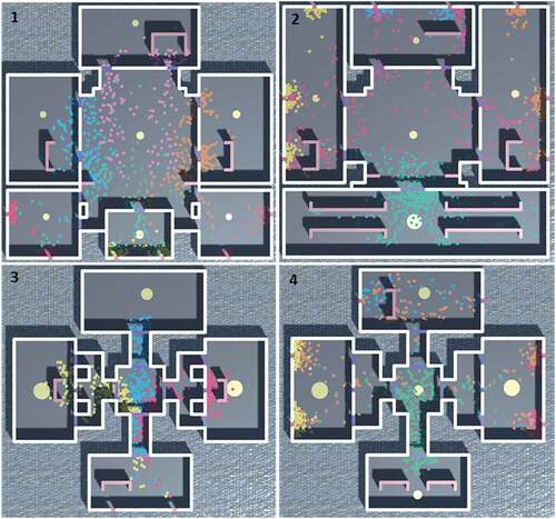
Figure 8. Still images from the visualisation of the numerical calculation processes for setups 5–8. A video visualisation of the simulation process associated with each setup can be viewed and/or downloaded from the links below. Note that the videos are corresponding to simulation at default/calibrated parameters, and not any deviation from the calibrated values.

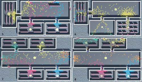
Table 4. The list of numerical simulation setups.

Setup No.	No. of rooms	No. of agents	No. of intermediate exits	No. of final exits	Dominant pattern of movement
1	7	850	11	6	Merge+Diverge
2	5	1000	7	8	Diverge
3	9	450	12	2	Merge
4	8	850	11	6	Diverge
5	5	1100	4	4	Merge
6	5	1100	4	6	Diverge
7	4	700	3	3	Merge
8	4	900	3	9	Diverge

Figure 9. Outcomes of the numerical analysis for the simulation setup 1. The variation of average of the total simulated evacuation time (denoted as Avg TET, shown with solid blue lines, presented on left vertical axes) as well as the average of the average individual evacuation time (denoted as Avg IET, shown with dotted red lines, presented on right vertical axes) associated with each parameter. The error bands represent standard deviation of the measurements. The horizontal access represents the value of the parameter through the scaling factor, η. At η=1, the simulation is performed with the calibrated value of the parameter.

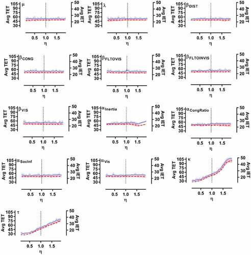
Figure 10. Outcomes of the numerical analysis for the simulation setup 2. The variation of average of the total simulated evacuation time (denoted as Avg TET, shown with solid blue lines, presented on left vertical axes) as well as the average of the average individual evacuation time (denoted as Avg IET, shown with dotted red lines, presented on right vertical axes) associated with each parameter. The error bands represent standard deviation of the measurements. The horizontal access represents the value of the parameter through the scaling factor, η. At η=1, the simulation is performed with the calibrated value of the parameter.

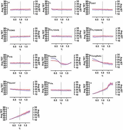
Figure 11. Outcomes of the numerical analysis for the simulation setup 3. The variation of average of the total simulated evacuation time (denoted as Avg TET, shown with solid blue lines, presented on left vertical axes) as well as the average of the average individual evacuation time (denoted as Avg IET, shown with dotted red lines, presented on right vertical axes) associated with each parameter. The error bands represent standard deviation of the measurements. The horizontal access represents the value of the parameter through the scaling factor, η. At η=1, the simulation is performed with the calibrated value of the parameter.

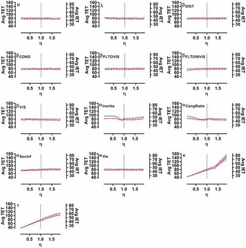
Figure 12. Outcomes of the numerical analysis for the simulation setup 4. The variation of average of the total simulated evacuation time (denoted as Avg TET, shown with solid blue lines, presented on left vertical axes) as well as the average of the average individual evacuation time (denoted as Avg IET, shown with dotted red lines, presented on right vertical axes) associated with each parameter. The error bands represent standard deviation of the measurements. The horizontal access represents the value of the parameter through the scaling factor, η. At η=1, the simulation is performed with the calibrated value of the parameter.

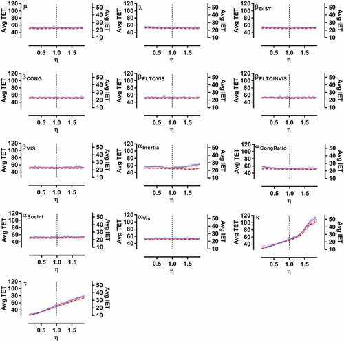
Figure 13. Outcomes of the numerical analysis for the simulation setup 5. The variation of average of the total simulated evacuation time (denoted as Avg TET, shown with solid blue lines, presented on left vertical axes) as well as the average of the average individual evacuation time (denoted as Avg IET, shown with dotted red lines, presented on right vertical axes) associated with each parameter. The error bands represent standard deviation of the measurements. The horizontal access represents the value of the parameter through the scaling factor, η. At η=1, the simulation is performed with the calibrated value of the parameter.

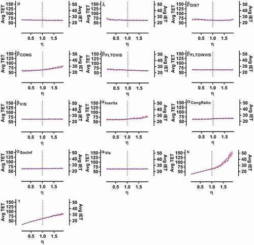
Figure 14. Outcomes of the numerical analysis for the simulation setup 6. The variation of average of the total simulated evacuation time (denoted as Avg TET, shown with solid blue lines, presented on left vertical axes) as well as the average of the average individual evacuation time (denoted as Avg IET, shown with dotted red lines, presented on right vertical axes) associated with each parameter. The error bands represent standard deviation of the measurements. The horizontal access represents the value of the parameter through the scaling factor, η. At η=1, the simulation is performed with the calibrated value of the parameter.

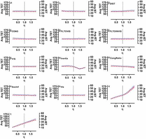
Figure 15. Outcomes of the numerical analysis for the simulation setup 7. The variation of average of the total simulated evacuation time (denoted as Avg TET, shown with solid blue lines, presented on left vertical axes) as well as the average of the average individual evacuation time (denoted as Avg IET, shown with dotted red lines, presented on right vertical axes) associated with each parameter. The error bands represent standard deviation of the measurements. The horizontal access represents the value of the parameter through the scaling factor, η. At η=1, the simulation is performed with the calibrated value of the parameter.

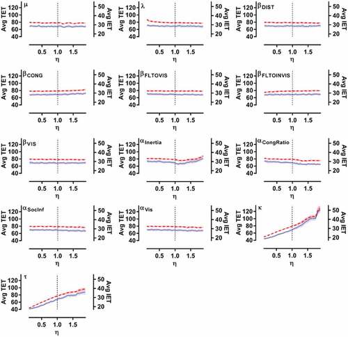
Figure 16. Outcomes of the numerical analysis for the simulation setup 8. The variation of average of the total simulated evacuation time (denoted as Avg TET, shown with solid blue lines, presented on left vertical axes) as well as the average of the average individual evacuation time (denoted as Avg IET, shown with dotted red lines, presented on right vertical axes) associated with each parameter. The error bands represent standard deviation of the measurements. The horizontal access represents the value of the parameter through the scaling factor, η. At η=1, the simulation is performed with the calibrated value of the parameter.

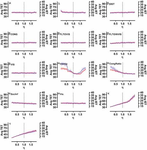
Figure 17. Outcomes of the numerical analysis for a selected subset of parameters (except for the social force parameters) to which the simulated evacuation times showed most amount of sensitivity in setups 1–5. The scale of the vertical axis has been adjusted and customised for each graph in order to better display the degree of variation.

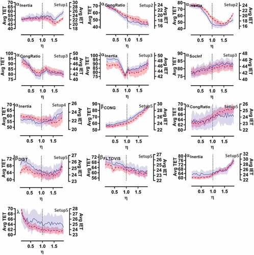
Figure 18. Outcomes of the numerical analysis for a selected subset of parameters (except for the social force parameters) to which the simulated evacuation times showed most amount of sensitivity in setups 6–8. The scale of the vertical axis has been adjusted and customised for each graph in order to better display the degree of variation.

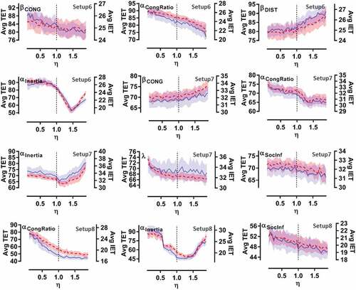
Figure A1 Visualization of the mass trajectories of simulated agents (subfigures (a)), maximum density (subfigures (b)), average density (subfigures (c)) and average velocity (subfigures (d)) for the simulation setups 1–4. The first component of each label signifies the number of the setup. The outputs are related to the calculations based on the default parameter setting of the numerical model.

Figure A2 Visualization of the mass trajectories of simulated agents (subfigures (a)), maximum density (subfigures (b)), average density (subfigures (c)) and average velocity (subfigures (d)) for the simulation setups 5–8. The first component of each label signifies the number of the setup. The outputs are related to the calculations based on the default parameter setting of the numerical model.

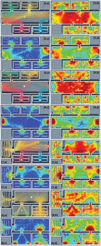
Figure A3 Legend for the heatmap plots in Figures A2 and A3.

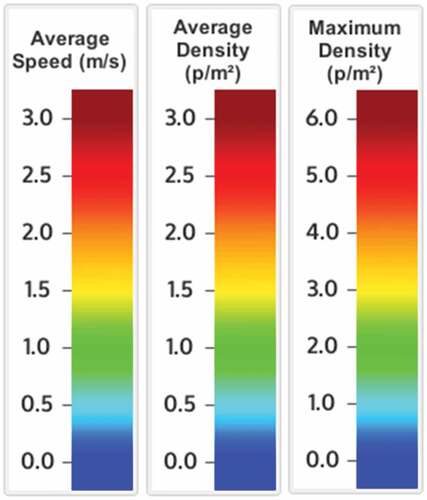
Figure A4 Three-dimensional visualization of the simulated evacuation process generated by the model for two example setups, with real-time path calculations (on the left) and the actual traversed trajectories (on the right) overlaid on the scene. Further videos demonstrating 3D visualisations of the simulation process can be downliaded from this link: https://unsw-my.sharepoint.com/:f:/g/personal/z3534847_ad_unsw_edu_au/EnRXneZRxQJAq9VGRkBqwq4BbFsqnUKYAfjYNLEHQolCQw?e=9SpyAD