Figures & data
Table 1. Image codification of the extrudates resulting from a mixture of coffee/sorghum/water.
Figure 1. (a) Image of the extrudates, (b) red, green, and blue (RGB) matrix distribution of colors, adapted from: https://www.dreamstime.com/stock-image-rgb-cmyk-color-cube-image27461991. (c) RGB matrix image. (d) Example of converting a red matrix into a column vector. (e) Transposition of the three vectors joined to form a one-row vector.
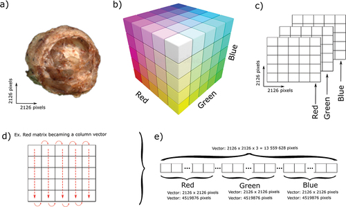
Figure 2. Images from 16 extrusion treatments from mixes of two sorghum genotypes, four coffee powder levels, and two moisture contents.
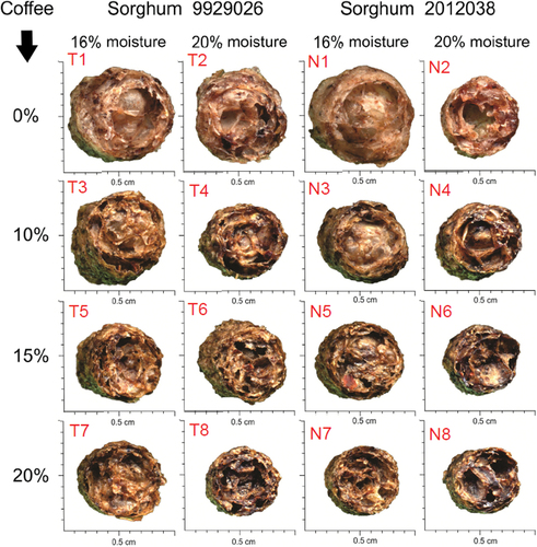
Figure 3. Scree plot of the 15 principal components obtained from the initial 13,559,628 variables.
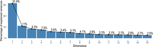
Figure 4. Principal component analysis of the original images (2126 x 2126 pixels), a) PC1 vs. PC2, b) PC3 vs. PC4.
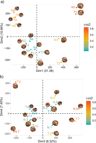
Figure 5. Dendrogram from hierarchical clustering of principal components (HCPC) for the 16 images.
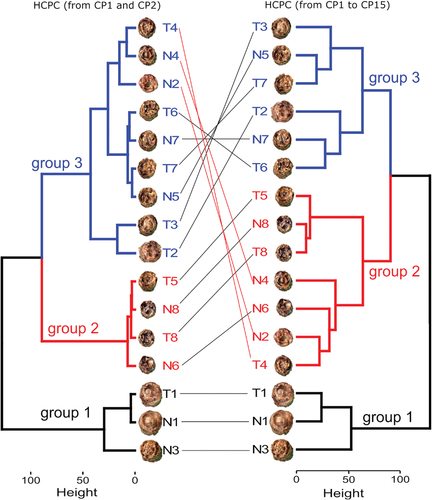
Figure 6. An example of the image reduction from the original size (2126 pixels).
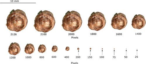
Figure 7. Percentage of the variance explained from the 15 PCs obtained applying the PCA technique for different image sizes (2126, 2100, 2000, 1800, 1600, 1400, 1200, 1000, 800, 600, 400, 200, 150, 100, 75, 50 and 25 pixels) using (a) color images and (b) grayscale images.
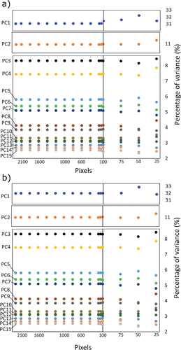
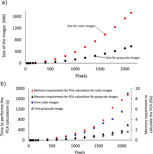
Figure 8. Computer memory requirements (a) to allocate the images, and (b) to carry out the PCA analysis. All calculations were performed using different image sizes (2126, 2100, 2000, 1800, 1600, 1400, 1200, 1000, 800, 600, 400, 200, 150, 100, 75, 50, and 25 pixels) using color and grayscale images.