Simulation of capillary infiltration into packing structures for the optimization of ceramic materials using the lattice Boltzmann method

Figures & data

Table 1. Relevant data for the packing structures composed of spheres.

Type	Diameter	Volume ()	Filling
bimodal1			0.46
bimodal2			0.46
bimodal3			0.46
multimodal			0.46
granular1	0.20	4.20	0.46
granular2	0.16	2.10	0.46
fine1	0.12	0.90	0.46
fine2	0.08	0.30	0.44

Note: Multiple values for the average size are given in the case of bimodal and multimodal mixtures. Figure 1 presents some 2D examples of the porous structures.

Table 2. Basic information for the porous systems obtained from the packing of rhombs.

Type	Side	Volume ()	Filling
bimodal1
bimodal2
bimodal3
multimodal
granular1	0.20	9.00
granular2	0.16	3.90
fine1	0.13	1.90
fine2	0.08	0.60

Note: The height of the rhombs is comparable to the length of their four equal sides, i.e. h=0.2,0.16,0.12,0.08. Bimodal and multimodal mixtures are characterized by multiple data for the size of the particles. The values for the filling fraction correspond to different orientations of the particles: aligned, misaligned, and misaligned and tilted, respectively. Figure 1 presents some 2D examples of the porous structures.

Table 3. Data for the packing structures obtained with fibers and rhombs.

Type	Side	Volume ()	Filling
fiber1
fiber2
fiber3
fiber4
fiber5
fiber6
fiber7
fiber8
fiber9

Note: For the side and the volume, the first value refers to the sticks and the second to the rhombs. For fibers, the side of the square base has a length of 0.06. The height of the rhombs is h=0.2,0.16,0.12,0.08, that is, similar to the length of the four equal sides. The reported filling fractions are associated with different orientations of the particles: aligned, misaligned, and misaligned and tilted, respectively. Figure 1 presents some 2D examples of the porous structures.

Figure 1. 2D sections for packing structures: (a) bimodal1 for spheres, (b) fine1 for spheres, (c) multimodal for blocks, (d) bimodal3 with misalignment for blocks, (e) fiber1 for misalignment, (f) fiber6 for misalignment and tilt, and (g) the microstructure of a typical preform.

Note: The filler particles are shown in the dark sections. Further information on the structures can be found in Tables 1 to 3.

Figure 2. Fluid invasion for selected packing structures after ts: (a) simulation for bimodal1 with spherical particles, (b) infiltration for bimodal2 with rhombs in the presence of misalignment, (c) visualization of a system using fiber2, with misalignment and tilt, and (d) simulation of bimodal2 for rhombs with misalignment and surface reaction enabled.

Note: Red is used for the wetting fluid and blue for the non-wetting component. The initial solid phase is represented by the dark areas and the growing surface from the reaction is represented by the yellow areas. More details on the properties of the packing systems are reported in Tables 1 to 3, and more details on the results of the infiltrations are reported in Tables 4 to 7.

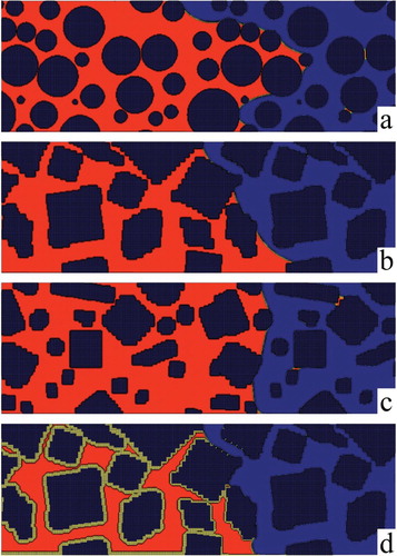
Figure 3. Infiltrated distance with chemical inertness for the solid surface: (a) packing structures obtained from spheres, and (b) packing structures realized with aligned rhombs.

Note: Points represent simulation results. The solid lines are fits to the data using Equation (3(3) ). The basic properties of the packing systems are listed in Tables 1 and 2.

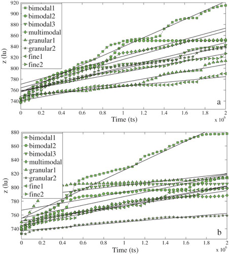
Table 4. Spheres composing the packing structures infiltrated without surface growth (see Table 1).

Type	(lu)	(lu/ts)	(lu/ts)	(lu)	K (lu^2)			Ca		Re
bimodal1		0.71	0.83	0.44	3.19	1.17	2.07	1.40	2.59	1.85
bimodal2		0.65	0.51	0.27	4.65	1.26	0.56	1.28	1.35	1.05
bimodal3		0.65	0.45	0.24	3.53	1.22	0.34	1.29	1.19	0.92
multimodal		0.79	0.52	0.27	2.22	1.24	0.26	1.58	2.06	1.30
granular1		1.09	0.33	0.17	2.10	1.34	0.11	2.16	2.46	1.14
granular2		0.75	0.41	0.21	1.80	1.17	0.19	1.49	1.44	0.97
fine1		0.41	0.18	0.09	1.08	1.30	0.90	0.82	0.19	0.23
fine2		0.74	0.34	0.18	0.97	1.18	0.27	1.46	1.17	0.80

Table 5. Rhombs composing the packing systems infiltrated with inert boundaries (see Table 2).

Type	(lu)			(lu/ts)	(lu/ts)	(lu)	K (lu^2)			Ca		Re
bimodal1
bimodal2
bimodal3
multimodal
granular1
granular2
fine1
fine2

Note: For every quantity, the multiple values correspond to the following different orientations of fillers: aligned, misaligned, and misaligned and tilted (see Figure 1).

Figure 4. Relationship between the fluctuations of characteristic numbers and Ca for packing systems with spheres and rhombs in the absence of surface reaction.

Note: Yellow markers are used for spheres, blue for aligned rhombs, red for rhombs with misalignment and green for rhombs with misalignment and tilt (see Tables 1 and 2).

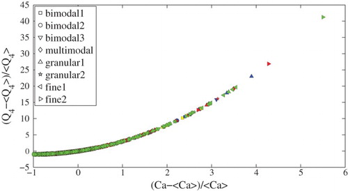
Figure 5. Relationship between the capillary number and the tortuosity for packing systems with spheres and rhombs in the absence of surface reaction.

Note: Yellow markers are used for spheres and blue for aligned rhombs. The properties of the packing systems are summarized in Tables 1 and 2.

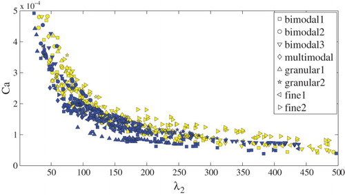
Table 6. Fibers added to the packing systems infiltrated without reactive boundaries (see Table 3).

Type	(lu)			(lu/ts)	(lu/ts)	(lu)	K (lu^2)			Ca		Re
fiber1
fiber2
fiber3
fiber4
fiber5
fiber6
fiber7
fiber8
fiber9

Note: For every quantity, the multiple values correspond to the following different orientations of fillers: aligned, misaligned, and misaligned and tilted (see Figure 1).

Table 7. Surface reaction enabled for the infiltration of packing systems obtained from rhombs (see Tables 2 and 5).

Type	(lu)	(lu/ts)	(lu)				Ca		Re
bimodal1
bimodal2
bimodal3
multimodal
granular1
granular2
fine1
fine2

Note: For every quantity, the multiple values correspond to the following different orientations of fillers: aligned, misaligned, and misaligned and tilted (see Figure 1).

Figure 6. Average maximum of the invading front as time passes for infiltrations with surface reaction.

Note: The porous structures are obtained from the packing of rhombs with aligned particles (see Table 2). Points represent simulation results. The solid lines are fits to the data by means of Equation (2(2) ).

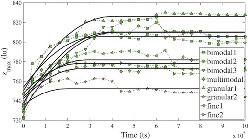
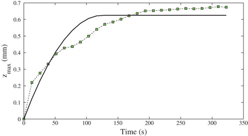
Figure 7. LBM simulations of the experimental results with surface growth.

Note: The average maximum for the infiltrated length is given as a function of time. Points represent simulation results. The solid line is a fit to the data by means of Equation (2(2) ).

Table 8. Characteristic dimensionless numbers for infiltrations in the presence of surface growth.

				Ca		Re
LBM systems
Real systems

Note: The results for LBM simulations are obtained from the systems with higher resolution leading to the results of Figure 7. In the case of real systems, typical experimental parameters are used (see section 5).