Numerical simulation of wind turbulence by DSRFG and identification of the aerodynamic admittance of bridge decks

Figures & data

Figure 1. Cross-sections of bridge decks: (a) Great Belt East Bridge, (b) Danjiang Reservoir Bridge (units: m).

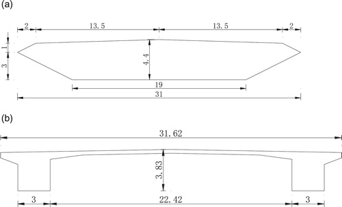
Figure 2. Computational domain and boundary conditions.

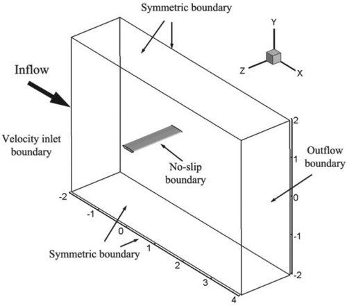
Figure 3. Meshing of the computational domain: (a) overview of the mesh arrangement, (b) distribution of the mesh near the streamlined box girder, (c) distribution of the mesh near the $\mathrm{\Pi }$ type girder.

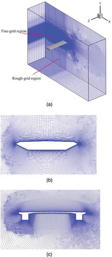
Figure 4. y⁺ distribution on girder surface: (a) Great Belt East Bridge, (b) Danjiang Reservoir Bridge.

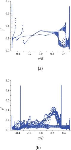
Figure 5. Workflow for the identification of the AAF of bridge decks.

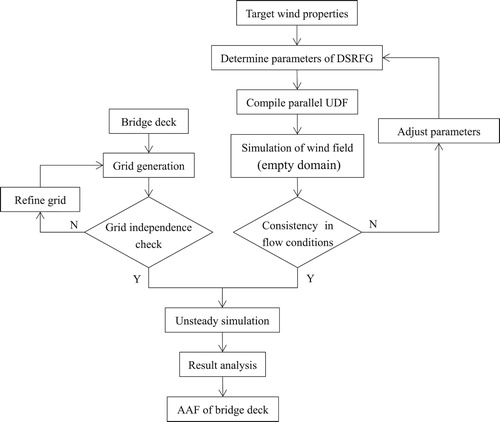
Table 1. Turbulence properties at the Great Belt East Bridge site.

Longitudinal turbulence intensity	Iu	10%
Vertical turbulence intensity	Iw	6%
Exponential decay factor	α	8

Figure 6. Comparison of the spatial correlation factors with different C_sp values: (a) u component, (b) v component, (c) w component.

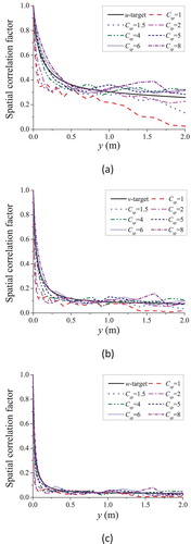
Figure 7. Simulated time histories of fluctuating wind velocity.

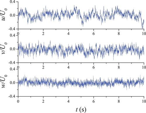
Figure 8. Simulated wind spectra in comparison with target spectra.

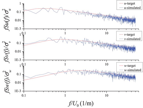
Table 2. Key parameters adopted in the DSRFG method.

M	N	dt	Csp
256	100	0.001s	5

Table 3. Simulated turbulent velocities for Great Belt East Bridge site in comparison with target values.

	Target value	Simulated value	Relative error
σu	1	1.011	1.1%
σv	0.88	0.873	0.8%
σw	0.6	0.577	3.8%

Figure 9. Mean wind velocity profiles in comparison with target profiles: (a) $\mathrm{\Delta }l$=2 cm, (b) $\mathrm{\Delta }l$=1 cm, (c) $\mathrm{\Delta }l$=0.5 cm.

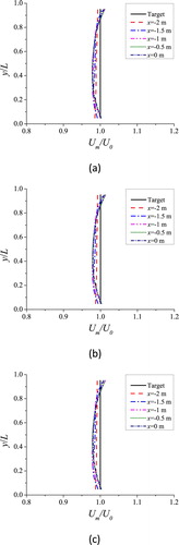
Figure 10. Turbulence intensity profiles in comparison with target profiles: (a) $\mathrm{\Delta }l$=2 cm, (b) $\mathrm{\Delta }l$=1 cm, (c) $\mathrm{\Delta }l$=0.5 cm.

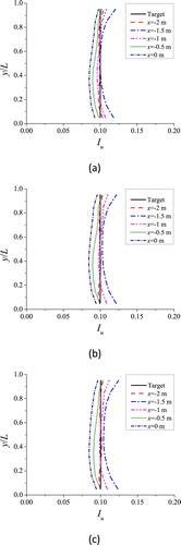
Figure 11. Spectra of the longitudinal velocity component in comparison with the target spectrum: (a) $\mathrm{\Delta }l$=2 cm, (b) $\mathrm{\Delta }l$=1 cm, (c) $\mathrm{\Delta }l$=0.5 cm.

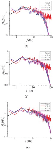
Figure 12. Spectra of the vertical velocity component in comparison with the target spectrum: (a) $\mathrm{\Delta }l$=2 cm, (b) $\mathrm{\Delta }l$=1 cm, (c) $\mathrm{\Delta }l$=0.5 cm.

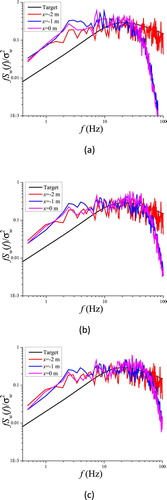
Figure 13. Turbulence integral scales in the computational domain.

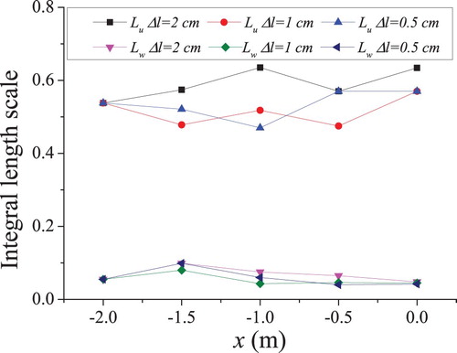
Figure 14. Wind spectra at x=2 m with different time step sizes in comparison with the target spectrum: (a) Spectra of the longitudinal velocity component, (b) Spectra of the vertical velocity component.

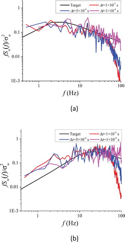
Figure 15. Turbulence kinetic energy contours.

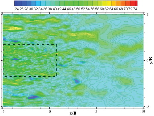
Figure 16. Vorticity magnitude contours.

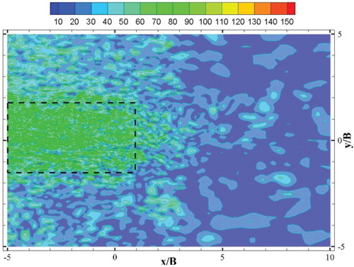
Figure 17. AAFs of a thin plate, (a) $|{\chi }_{Lu}{|}^2$, (b) $|{\chi }_{Mu}{|}^2$, (c) $|{\chi }_{Lw}{|}^2$ (d) $|{\chi }_{Mw}{|}^2$.

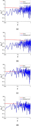
Figure 18. Arrangement of the monitoring points: (a) Great Belt East Bridge, (b) Danjiang Reservoir Bridge.

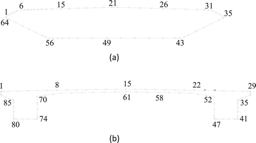
Figure 19. Mean pressure distribution, (a) upper surface of the Great Belt East Bridge, (b) lower surface of the Great Belt East Bridge, (c) Danjiang Reservoir Bridge.

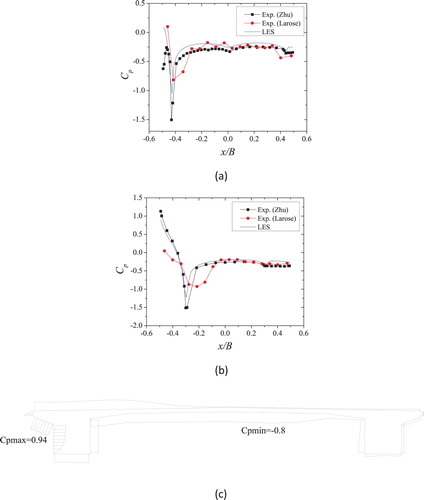
Figure 20. Instantaneous pressure contours around girder section: (a) Great Belt East Bridge, (b) Danjiang Reservoir Bridge.

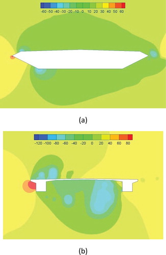
Figure 21. Streamlines of flow around the girder section: (a) Great Belt East Bridge, (b) Danjiang Reservoir Bridge.

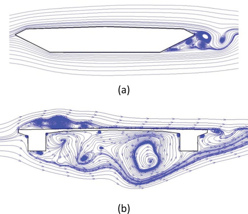
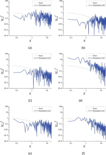
Figure 22. AAFs of the Great Belt East Bridge box girder section. The estimated vortex shedding frequency is indicated by a vertical line (dashed red). (a) $|{\chi }_{Lu}{|}^2$, (b) $|{\chi }_{Du}{|}^2$, (c) $|{\chi }_{Mu}{|}^2$, (d) $|{\chi }_{Lw}{|}^2$, (e) $|{\chi }_{Dw}{|}^2$, (f) $|{\chi }_{Mw}{|}^2$.

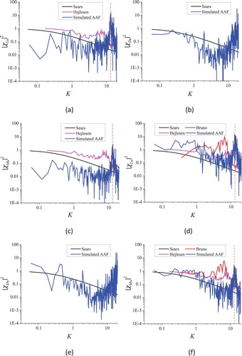
Figure 23. Spectral analysis of the lift time histories of the girder section at zero angle of attack.

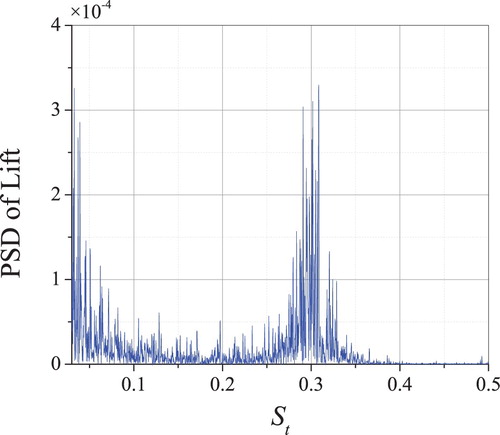
Figure 24. AAFs of the Danjiang Reservoir Bridge box girder section: (a) $|{\chi }_{Lu}{|}^2$, (b) $|{\chi }_{Du}{|}^2$, (c) $|{\chi }_{Mu}{|}^2$, (d) $|{\chi }_{Lw}{|}^2$, (e) $|{\chi }_{Dw}{|}^2$, (f) $|{\chi }_{Mw}{|}^2$.