Two-dimensional smoothed particle hydrodynamics (SPH) simulation of multiphase melting flows and associated interface behavior

Figures & data

Figure 1. Computational domain.

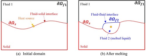
Figure 2. Illustration of (a) wetting and (b) non-wetting effects of the solid surface by melted liquids.

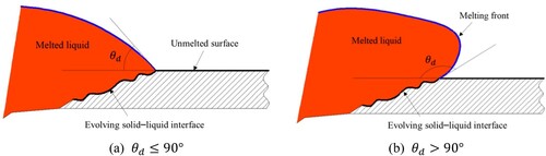
Figure 3. Particle distribution within the support domain of the smoothing function W for particle i. The support domain (${\mathrm{\Omega }}_{{\mathit{x}}_{\mathit{i}}}$) and its boundary S is circular with the radius of $ϵh$. The figure is cited from the book by Liu & Liu, 2003.

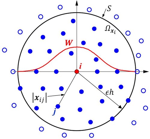
Figure 4. Illustration of particles near the interface.

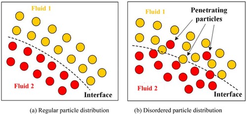
Figure 5. Treatment for new interface particles for considering the wetting effect.

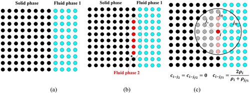
Table 1. Pseudo-code of implementing the established SPH model.

Initialization of SPH particles of the computational domain
Entering the time integration loop
1	Determining the artificial sound speed of each phase (Equations (9), and (10)).
2	Calculating the time step size $\mathrm{\Delta }t$ (Equations (56) and (57)).
3	Calculating the pressure p of each SPH particle according to the equation of state (Equations (6) and (7)).
4	Generating boundary particles and assigns the variable value to each boundary particle according to no-slip or free-slip boundaries.
5	Searching neighboring particles using the linked-list method, and establishing the index array of neighboring particle pairs.
6	Calculating the values of kernel function and kernel gradient for each neighboring particle pair (Equation (27)).
7	Identifying all interface particles, and calculating the normal vector and the curvature for each interface particle (Equations (44) and (47)).
8	Calculating the surface tension force and the interface sharpness force for each interface particle (Equations (48) and (49)).
9	Calculating the pressure gradient term and the viscous force term for each fluid particle (Equations (38) and (40)).
10	Calculating the density for each fluid particle (Equation (37)).
11	Calculating the acceleration of each fluid particle.
12	Updating the velocity, position, and temperature of each particle (Equations (54) and (55)).
13	Setting the specific heat capacity of the particle which is located in the temperature range between $T_m-\mathrm{\Delta }T$ and $T_m+\mathrm{\Delta }T$ (Equation (2)).
14	Calculating the rate of temperature for each fluid particle (Equation (24)).
15	Calculating the acceleration of each fluid particle.
16	According to the temperature range of the particle, triggering the transition of phase state of the concerned particle.
17	If the current time step n+1 is less than the terminal time step, returning to 1
End

Figure 6. Schematic of the one-phase Stefan problem (benchmark example 1).

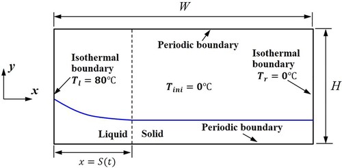
Figure 7. Illustration of phase interface and temperature distribution at the time 55.5 s.

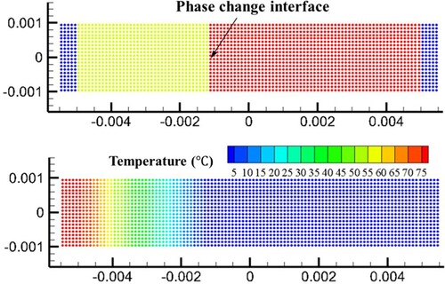
Figure 8. The time history of the phase interface position for various temperature interval $\mathrm{\Delta }T$.

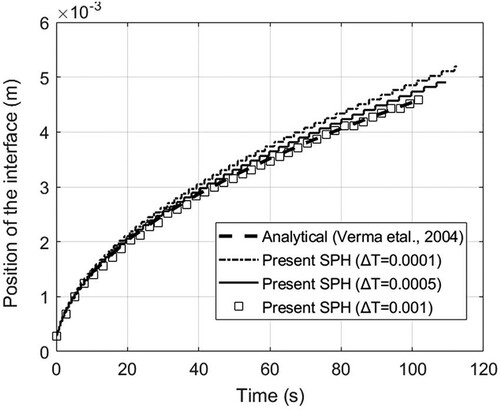
Figure 9. Model parameters and SPH model (benchmark example 2).

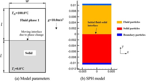
Figure 10. Simulation results of evolution of solid–liquid interface due to phase change.

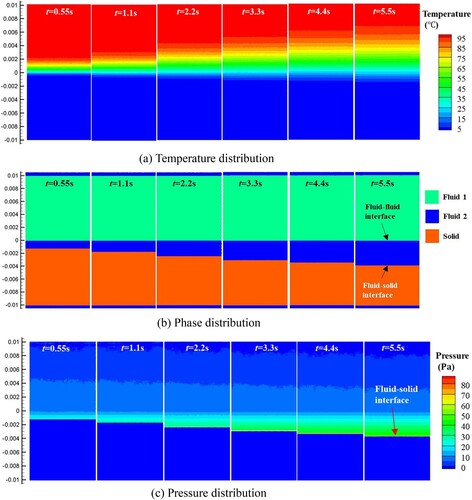
Figure 11. Temperature distributions along vertical (y) direction at different time instants.

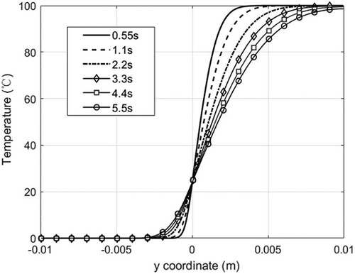
Figure 12. Pressure distributions along vertical (y) direction.

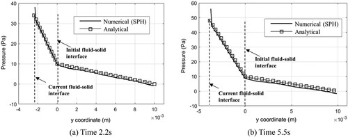
Figure 13. (a) The initial particle distribution for the test of square droplet deformation, and (b) the particle distribution at t = 6.0s.

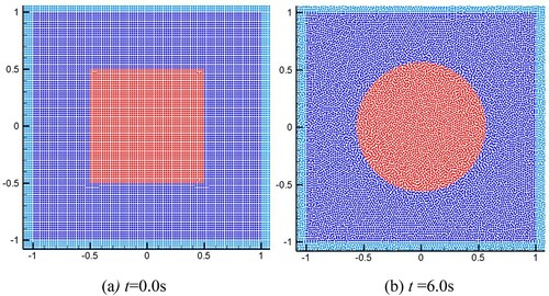
Figure 14. Time history of pressure difference. (a) Density ratio (DR) = 1.0, showing effect of smoothing length. (b) DR = 100.0, showing effect of interface sharpness force ($\zeta$).

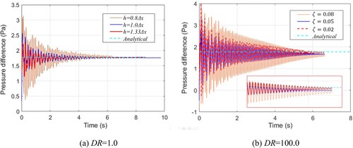
Figure 15. Pressure distributions using various smoothing lengths.

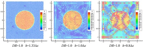
Figure 16. Pressure distributions using different ζ.

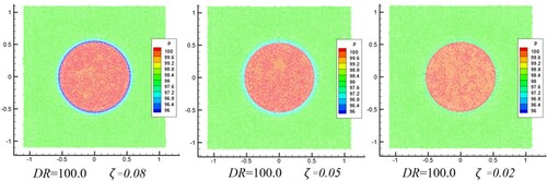
Figure 17. (a) Model parameters of single bubble rising, and SPH results of stable bubble based on different particle spacing: (b) $\mathrm{\Delta }x=R/25.0$; (c) $\mathrm{\Delta }x=R/18.75$; (d) Bubble profiles at different time instants.

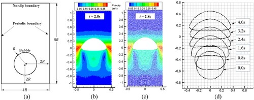
Table 2. Parameters for single bubble rising (model validation).

Fluid	Density (kg/m^3)	Viscosity (N·s/m^2)	Droplet diameter (m)	Surface tension coefficient (N/m)	Gravity acceleration (m/s^2)
Heavy phase	1000.0	10.0	0.25	24.5	0.98
Light phase	100.0	1.0

Figure 18. (a) Time history of velocity of ascending bubble, and (b) terminal bubble morphologies using different particle spacings (t = 2.8s).

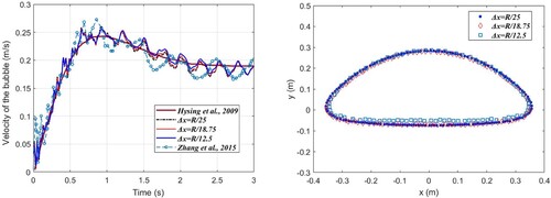
Table 3. Physical parameters for two rising bubbles.

Fluid	Density (kg/m^3)	Viscosity (N·s/m^2)
l	1000.0	0.156
g	100.0	0.078

Figure 19. Schematic of two rising bubbles.

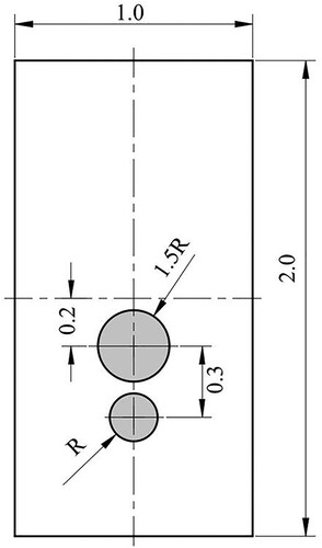
Figure 20. SPH results of two rising bubbles (Bo = 80.0).

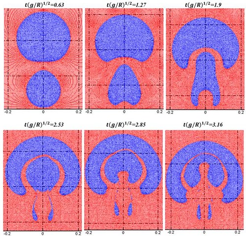
Figure 21. SPH results of two rising bubbles, showing the velocity distribution (Bo = 80.0).

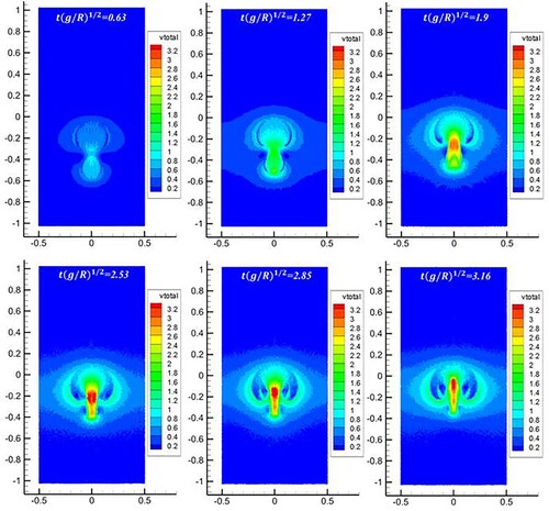
Figure 22. Comparison of bubble morphologies between present SPH results (blue line) and level-set results (dotted red line, Grenier et al., 2013) (Bo = 80.0).

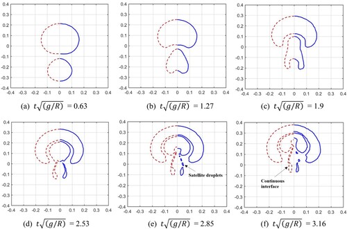
Figure 23. Schematic of melting of a square solid (case 1).

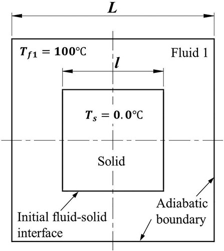
Figure 24. The time history of melted liquid volume with three particle resolutions. The volume is obtained by multiplying the area of molten liquid by the reference length (1.0m).

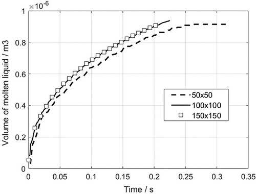
Figure 25. Simulation result of the melting process of a square solid (case 1).

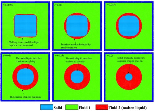
Figure 26. Temperature distributions at different time instants (case 1).

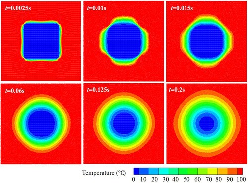
Figure 27. The particle distribution and normal vector of the interface at the initial moment of melting (t = 0.0025s).

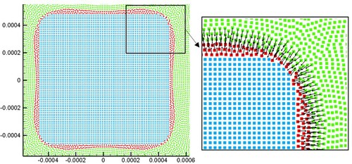
Figure 28. Model parameters of a square solid melting on an adiabatic wall (case 2).

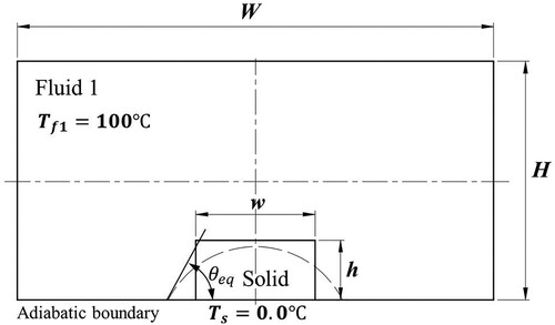
Figure 29. (a) Comparison of droplet morphologies between two particle resolutions (t = 0.18 s), (b) trends of melted liquid volume are obtained using three particle resolutions. The volume is obtained by multiplying the area of molten liquid by the reference length (1.0m).

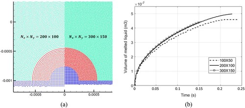
Figure 30. Simulation results of the melting process of a square solid on an adiabatic wall (case 2).

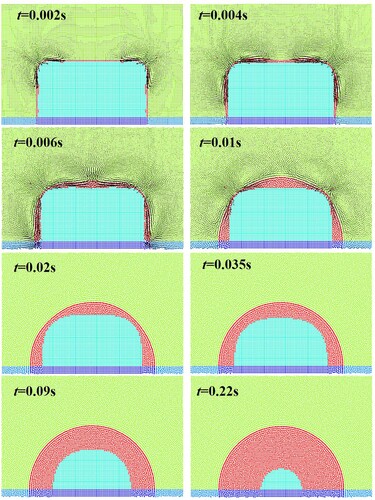
Figure 31. Temperature distributions at different times (case 2).

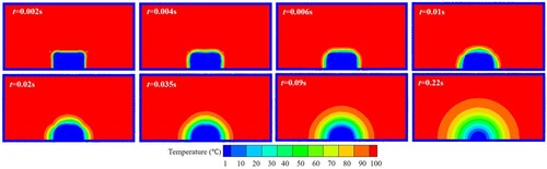
Figure 32. Model parameters and initial conditions of sinking and melting of a square solid (case 3).

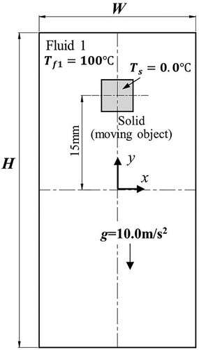
Figure 33. Time history of melted liquid volume using three different particle resolutions (case 3). The volume is obtained by multiplying the area of molten liquid by the reference length (1.0m).

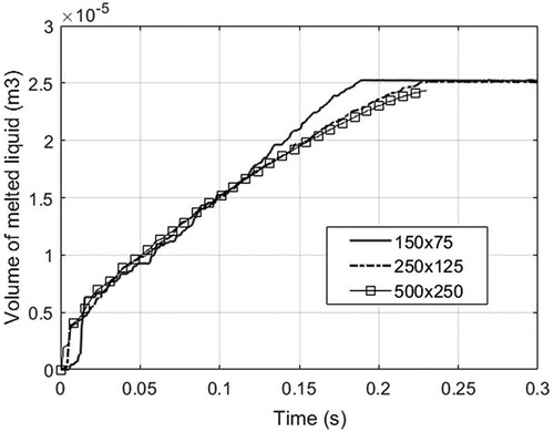
Figure 34. Comparison of droplet morphology between two different resolutions.

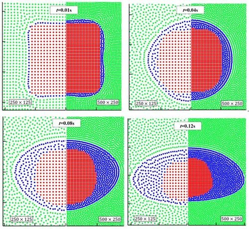
Figure 35. SPH results of sinking and melting process of an initially square solid.

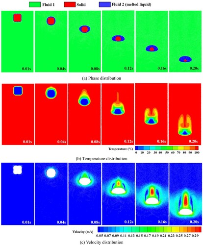
Figure 36. Temperature distribution inside the droplet during sinking of the solid. The morphology of the (unmelted) solid is shown in white (case 3).

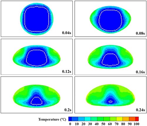
Figure 37. Initial temperature distributions for case 4.

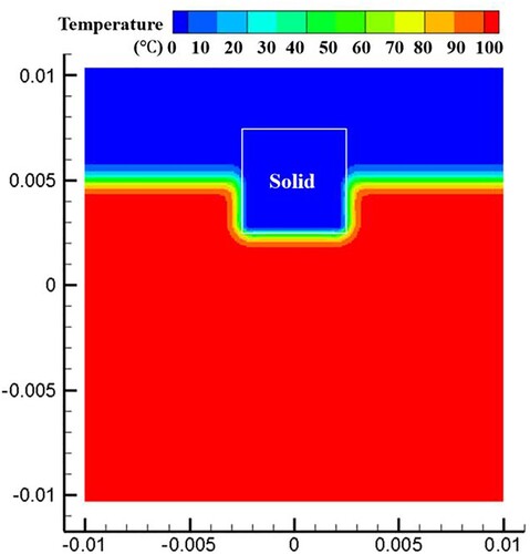
Figure 38. (a) Time evolution of melted liquid volume with four different particle resolutions, (b) comparison of the droplet profile between two particle resolutions at time 0.22 s (the convergence study for case 4). The volume is obtained by multiplying the area of molten liquid by the reference length (1.0m).

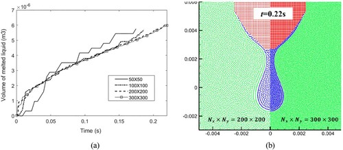
Figure 39. Simulation results of molten droplet formation and dripping process (case 4).

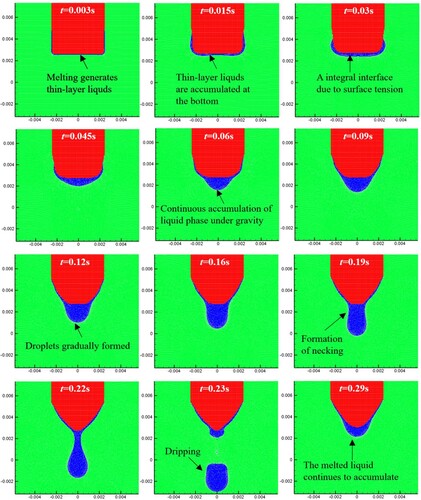
Figure 40. The temperature distribution at different time instants (case 4).

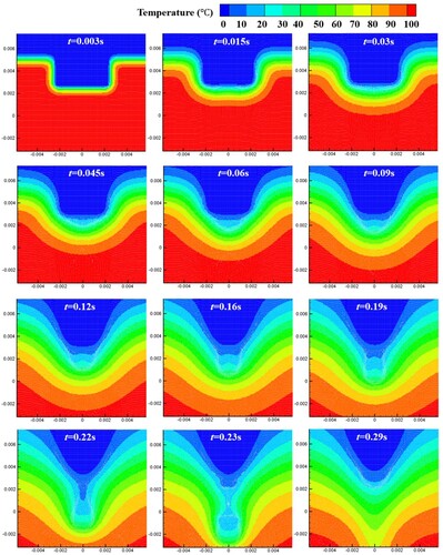
Figure 41. Droplet fragment. Arrows denote the interface normal vector.

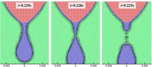
Figure 42. Results of molten droplet formation and dripping process for the three different Bond numbers.

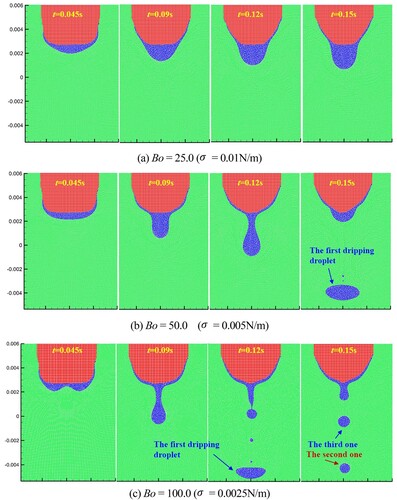
Figure 43. The time curve of melted liquid (a) volume and (b) melt kinetic energy with respect to different Bond numbers. The volume is obtained by multiplying the area of molten liquid by the reference length (1.0m).

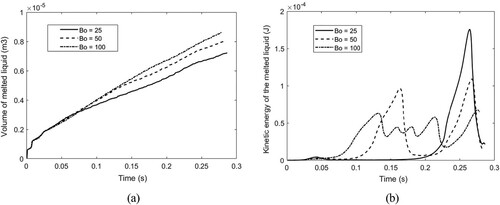
Figure 44. Initial model of wax melting (case 5).

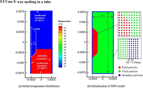
Figure 45. Simulation results of wax melting process.

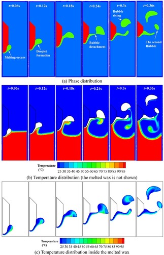
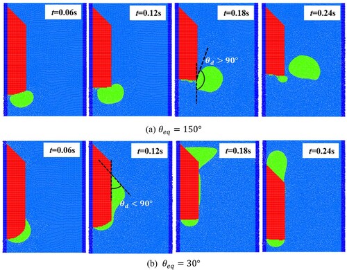
Figure 46. Effect of Bond number on interface behaviors of melted wax.

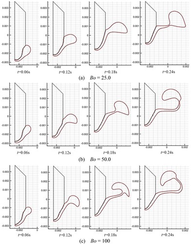
Figure 47. The solid surface is (a) not wetted or (b) wetted by the melted liquid.

Liu, G. R., & Liu, M. B. (2003). Smoothed particle hydrodynamics: A meshfree particle method. World Scientific.

 Google Scholar

Grenier, N., Le Touzé, D., Colagrossi, A., Antuono, M., & Colicchio, G. (2013). Viscous bubbly flows simulation with an interface SPH model. Ocean Engineering, 69, 88–102. https://doi.org/10.1016/j.oceaneng.2013.05.010

 Web of Science ®Google Scholar