Figures & data
Figure 1. Hybrid noise prediction procedure. 3D = three-dimensional; CFD = computational fluid dynamics; DES = detached eddy simulation; CAA = computational aeroacoustics; FEM = finite element method; APML = adaptive perfectly matched layer.
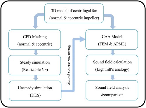
Figure 2. Overview of the three-dimensional high-speed centrifugal fan model.
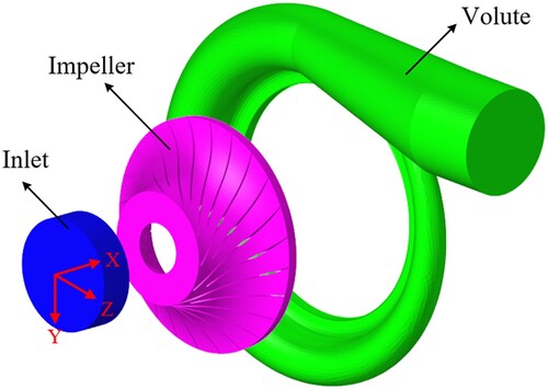
Table 1. Parameters of the centrifugal fan.
Figure 3. Comparison of the total pressure of the normal case obtained by Spalart–Allmaras (S-A) delayed detached eddy simulation (DDES) and realizable k-ε (RKE) DDES. Cal. = calculated; Exp. = experimental.
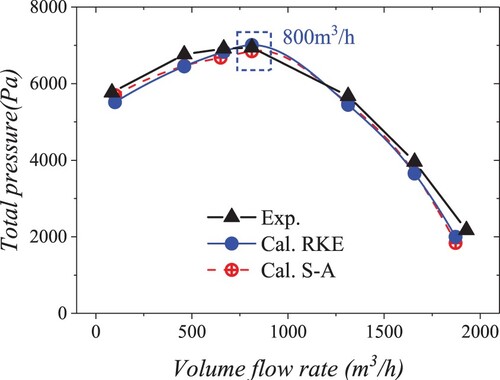
Figure 4. Diagram of the impeller motion model considering the eccentric effect.
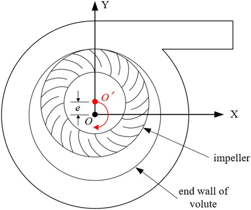
Figure 5. Pressure rises with different extension lengths of the pipes. Cal. = calculated; Exp. = experimental.
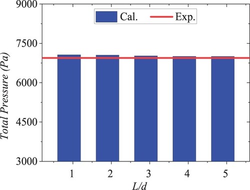
Figure 6. Computational fluid dynamics (CFD) mesh in different domains: (a) impeller mesh; (b) wall mesh of impeller; (c) boundary layer of impeller; (d) cut plane of volute mesh.
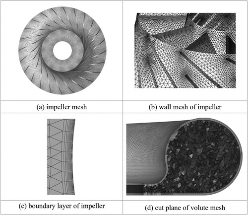
Figure 7. Mesh independence analysis. Exp. = experimental.
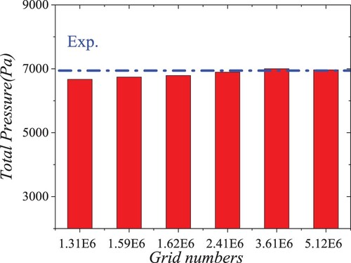
Figure 8. The y-plus distribution.
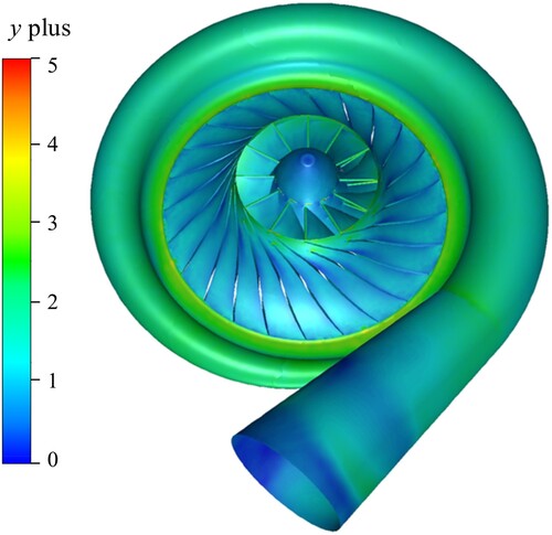
Table 2. Computational fluid dynamics settings.
Figure 9. Computational aeroacoustic (CAA) model for a high-speed centrifugal fan. APML = adaptive perfectly matched layer.
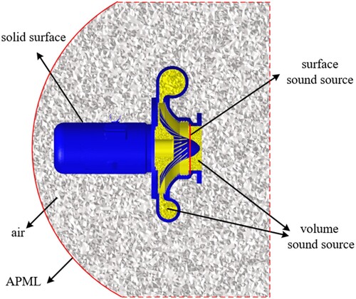
Figure 10. Test bench settings: (a) distribution of acoustic transducers; (b) B&K 4957 microphone; (c) experimental layout.
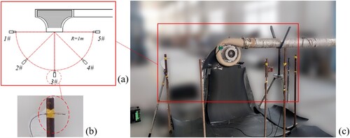
Figure 11. Comparison of calculated (Cal.) and experimental (Exp.) performance curves: (a) total pressure; (b) internal efficiency.
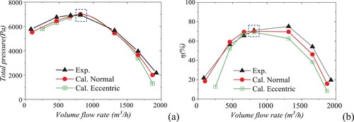
Figure 12. Velocity vector comparison.
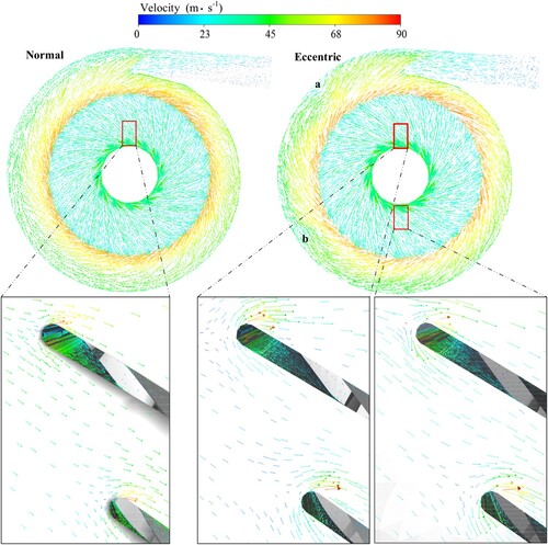
Figure 13. Pressure contour on the span plane at (a) 10%, (b) 50%, and (c) 90% blade height.
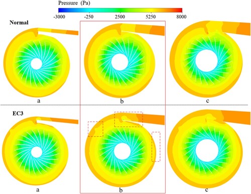
Figure 14. Blade loading comparison for 0–0.2 chord length (50% blade height).
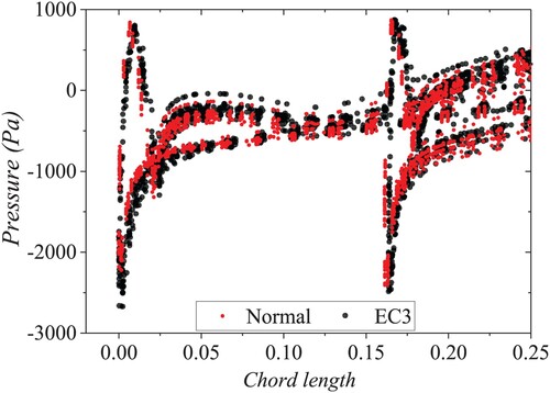
Figure 15. Turbulence kinetic energy distribution comparison (50% blade height span plane).
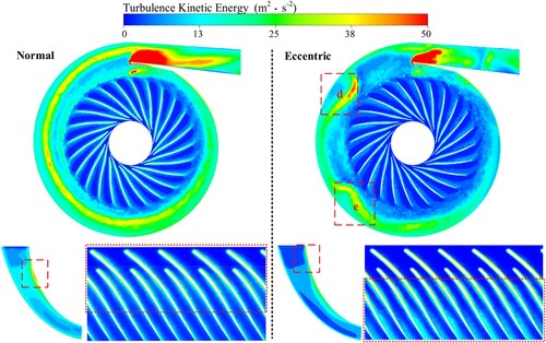
Figure 16. Inlet mass and outlet pressure in 10 rounds: (a) inlet mass comparison; (b) outlet total pressure; (c) inlet mass fluctuation at the second blade passing frequency (BPF) in the normal case; (d) outlet pressure fluctuation at the second BPF in the normal case.
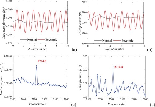
Figure 17. Setting of monitoring points.
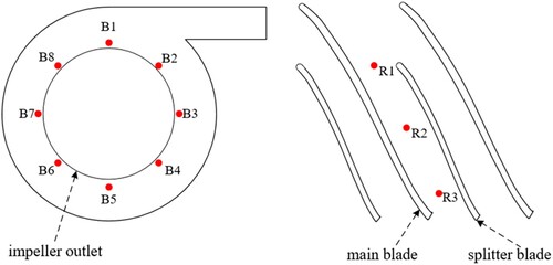
Figure 18. Pressure fluctuation at measuring points (MPs) in the frequency domain: (a) impeller passage; (b) normal impeller outlet; (c) eccentric impeller outlet; (d) impeller outlet with different eccentricities.
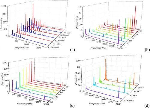
Figure 19. Variation of blade loading in one spin of the impeller (0–0.2 chord length): (a) blade loading range comparison for 0–0.2 chord length; (b) pressure contour at the leading edge of the eccentric impeller in one spin.
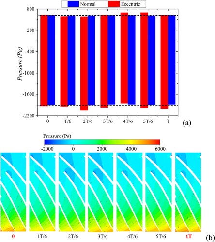
Figure 20. Vortex generation in the impeller with different instants.
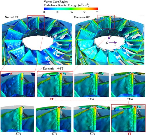
Figure 21. Vortex structure comparison in one round.
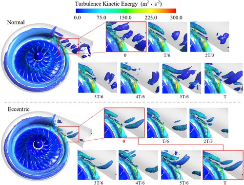
Figure 22. Frequency domain results at computational fluid dynamics (CFD) monitoring points: (a) experimental result at measuring points (MPs) 1–5; (b) calculated result at MPs 1–5; (c) noise spectrum comparison with finer computational aeroacoustic (CAA) mesh at monitoring point NO.3. SPL = sound pressure level.
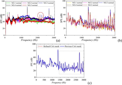
Figure 23. Comparison between calculated (Cal.) and experimental (Exp.) results of a normal impeller at measuring points (MPs) 1–5: (a) NO.1; (b) NO.2; (c) NO.3; (d) NO.4; (e) NO.5; (f) overall sound pressure level (OSPL) comparison at MPs 1–5. RF = rotating frequency; SPL = sound pressure level.
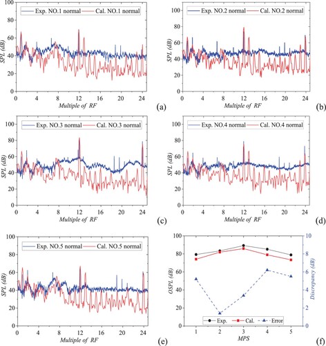
Figure 24. Sound directivity in the normal case. RF = rotating frequency; BPF = blade passing frequency; SPL = sound pressure level.
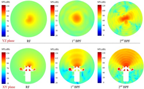
Figure 25. Overall sound pressure level (OSPL) results at measuring points (MPs) 1–5 under different impeller eccentricities.
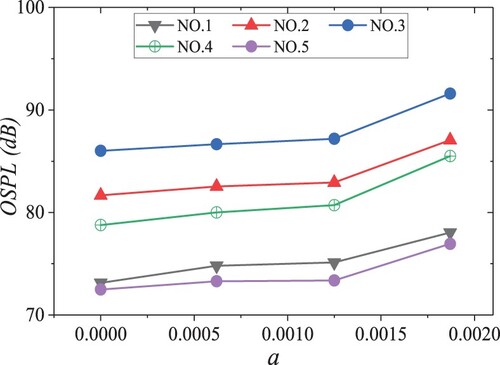
Figure 26. Frequency spectrum with an eccentric impeller at measuring points (MPs) 1–5: (a) experimental results; (b) calculated results. SPL = sound pressure level.
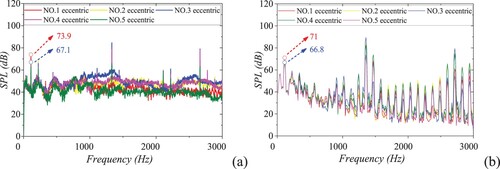
Figure 27. Total overall sound pressure level (OSPL) with an eccentric impeller at measuring points (MPs) 1–5.
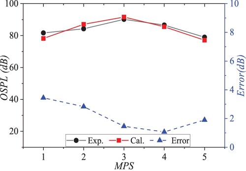
Figure 28. Eccentric effect on NO.4 noise spectrum: (a) experimental (Exp.) results; (b) calculated (Cal.) results. RF = rotating frequency; SPL = sound pressure level.
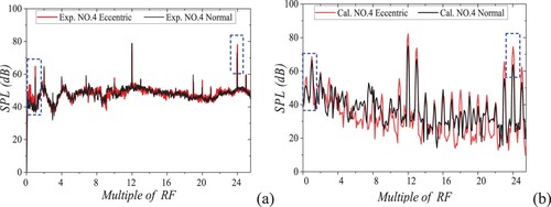
Figure 29. Experimental (Exp.) and calculated (Cal.) results at NO.4 (eccentric impeller). RF = rotating frequency; SPL = sound pressure level.
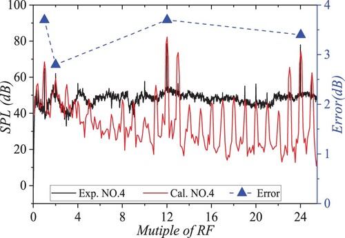
Figure 30. Noise spectrum at NO.4 measuring point with different impeller eccentricities: (a) noise spectrum at the whole frequency range; (b) partial result at rotating frequency (RF); (c) partial result at first blade passing frequency (BPF); (d) partial result at second BPF. SPL = sound pressure level.
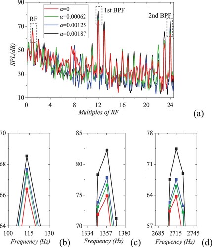
Figure 31. Eccentric effect on sound directivity at the second blade passing frequency (BPF). SPL = sound pressure level.
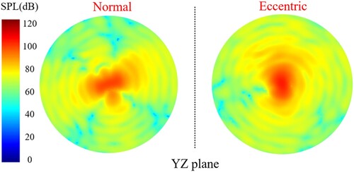
Figure 32. Lighthill’s surface contribution with an eccentric impeller. RF = rotating frequency; BPF = blade passing frequency.
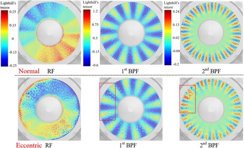
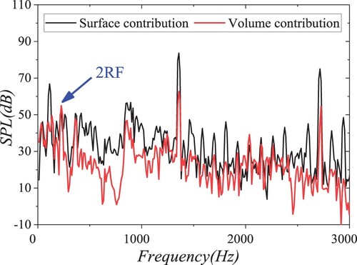
Figure 33. Sound source contribution with a normal impeller at NO.3 measuring point. RF = rotating frequency; SPL = sound pressure level.