Effect of multihole baffle-induced lobe flow structures on a high efficiency micro-thermophotovoltaic system

Figures & data

Figure 1. Schematic of the present micro combustor combined with micro-thermophotovoltaic.

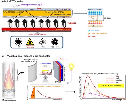
Figure 2. Computational domain and different baffle plates.

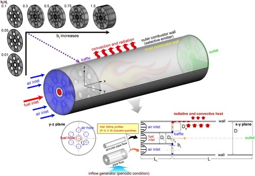
Table 1. Geometric conditions.

Parameter	Value (mm)
Air hole diameter, Da	0.40
Baffle thickness, bt	0.004–0.6
Combustor length, L	40.0
Fuel hole diameter, Df	0.40
Inner inflow tube diameter, Di	0.62
Inflow tube length, Li	5.60
Inner combustor diameter, D	2.80
Outer combustor diameter, Do	3.60
Radial air hole position, ra	0.80

Table 2. Inlet conditions of ϕ_G = 1.0.

	Um (m/s)	Ufuel/Uair	Mfuel/Mair	ReD	Refuel	Reair
CH4	38.245	4.909	0.287	500	917	1483
H2	88.319	18.934	0.549	500	352	889

Notes: Re_fuel= ${\rho }_{fuel}{D}_f{U}_{fuel}/{\mu }_{fuel}$, Re_air= ${\rho }_{air}{D}_a{U}_{air}/{\mu }_{air}$, M_fuel= ${\rho }_{fuel}\pi D_f^2{U}_{fuel}^2/4$, M_air= ${\rho }_{air}\pi D_a^2{U}_{air}^2/4$, ${\rho }_{C{H}_4}=0.6517\text{kg/}{\text{m}}^3$, ${\mu }_{C{H}_4}=1.09\times {10}^{-5}\text{kg/m}\cdot \text{s}$, ${\rho }_{air}=1.1709\text{kg/}{\text{m}}^3$, ${\mu }_{air}=1.7219\times {10}^{-5}\text{kg/m}\cdot \text{s}$.

Table 3. Boundary conditions of multihole baffled micro combustor.

Boundary	Parameters	Values
Inlet	Constant mass flow rate	$m_{in}^{\mathrm{\prime }C{H}_4}$ = 3.1321 × 10^−6 kg/s, $m_{in}^{\mathrm{\prime }air}$ = 5.35896 × 10^−5 kg/s
		$m_{in}^{\mathrm{\prime }{H}_2}$ = 9.3005 × 10^−7 kg/s, $m_{in}^{\mathrm{\prime }air}$ = 3.20867 × 10^−5 kg/s
Outlet	Pressure outlet	P = Pout = 101,325 Pa
Inner wall	Conjugate heat transfer	${\lambda }_{fluid}(\mathrm{\partial }T/\mathrm{\partial }{x}_i{)}_{fluid}=-{\lambda }_w(\mathrm{\partial }T/\mathrm{\partial }{x}_i{)}_w$
Outer wall	Radiation and convection	$q=h_w(T_w-T_{\mathrm{\infty }})+ϵ\sigma (T_w^4-T_{\mathrm{\infty }}^4)$
Solid zone	Stainless steel	ρ = 83,100 kg/m^3, Cp = 275 J/kgK, k = 92 W/mK

Table 4. Comparison of CH₄–air and H₂–air combustion.

Properties (ϕG = 1.0, P = 1 atm, T = 298 K)	CH4–air	H2–air
Density (kg/m^3)	0.668	0.0838
Molecular weight (kg/Kmol)	16.043	2.016
Air–fuel ratio	17.11	34.33
Stoichoimetic mixture fraction	0.055	0.02
High heating value (MJ/kg)	55.5	141.9
Adiabatic flame temperature (K)	2226	2400

Figure 3. Comparison of the flame length error for different CVs.

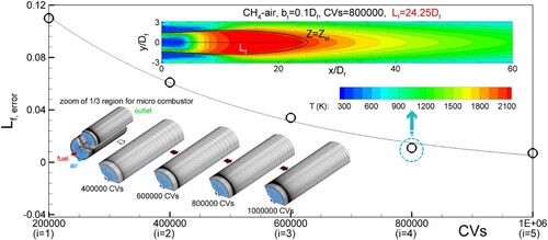
Figure 4. Comparison of temperature profiles along center axis between predicted result and experimental data: dependency of (b) turbulence models, and (c) chemical kinetic models.

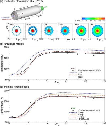
Figure 5. Recirculation zone characteristics, 3D contours, and axial distributions along the centerline of streamwise velocity (b_t= 0.1D_f).

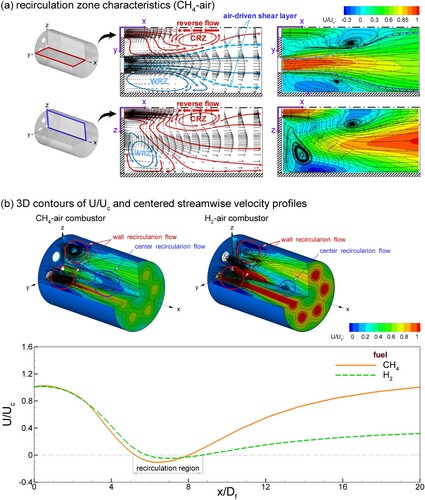
Figure 6. Velocity vectors and temperature contours (CH₄–air, b_t= 0.1D_f) The black solid line represents Z = Z_st.

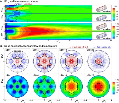
Figure 7. Comparisons of streamwise and azimuthal vorticities at x/D_f= 1.0, 2.0, 4.0, and 8.0 (b_t= 0.1D_f).

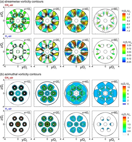
Figure 8. Streamwise vorticity magnitude variation with streamwise vorticity contours of AOA’ plane (CH4–air, b_t= 0.1D_f).

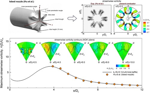
Figure 9. Temperature contours at several streamwise locations with iso-surface contour of Z = Z_st (CH₄–air and H₂–air, b_t= 0.1D_f).

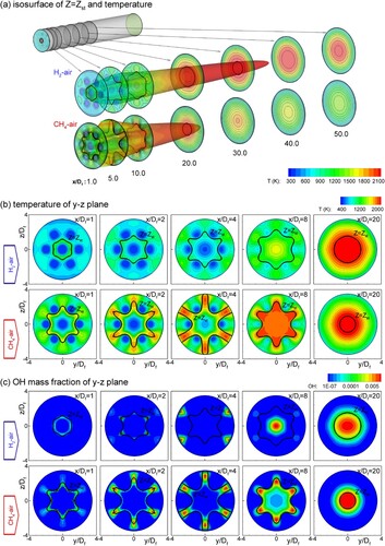
Figure 10. Axial distributions of temperature and mass fractions of reactants and products (CH₄–air and H₂–air, b_t= 0.1D_f).

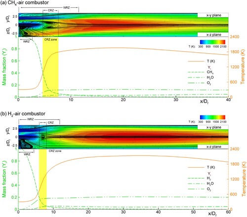
Figure 11. Streamlines, velocity vectors, and contours of temperature and OH mass fraction for different baffle conditions (CH₄–air, b_t= 0.1D_f).

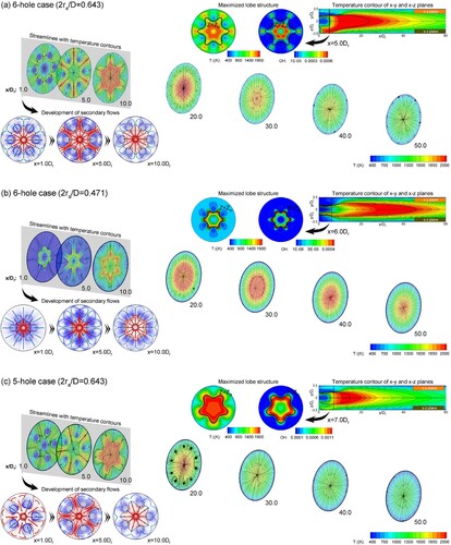
Figure 12. Schematic of secondary flows, velocity vectors, and streamwise vorticity contours.

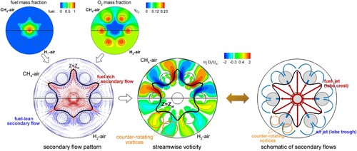
Figure 13. Comparisons of lobe intensity and wall friction coefficient (CH₄–air and H₂–air, b_t= 0.1D_f).

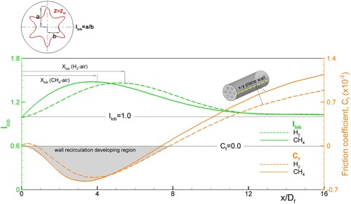
Figure 14. Evolution of the lobed structure and secondary flows.

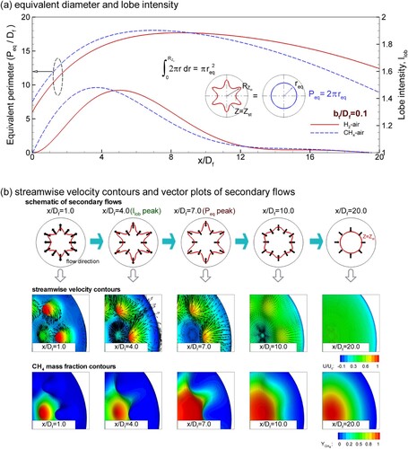
Figure 15. Variation of maximized vorticities and I_lob for different baffle thickness (CH₄–air).

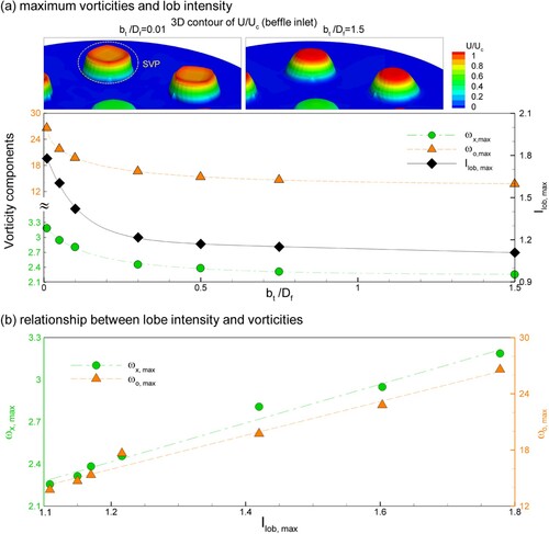
Figure 16. Comparison of probability density distributions of ${\varphi }_{local}$ and the summated PDF.

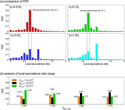
Figure 17. Temperature contours and azimuthally averaged wall temperatures for different b_t.

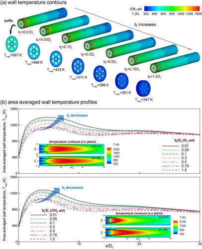
Figure 18. Variations of maximized I_lob location and heat loss depending on I_{lob, max}.

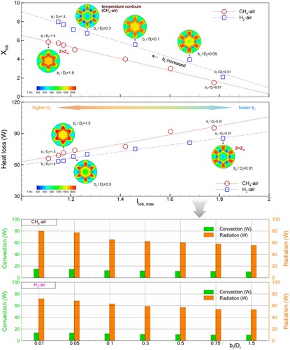
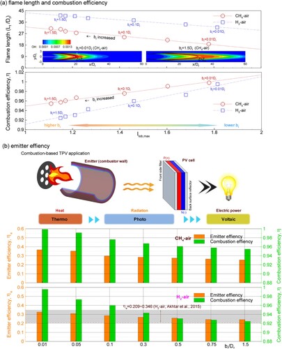
Figure 19. Variations of flame length and conversion rate depending on I_{lob, max}.