Effect of model scale and airflow velocity on aerodynamic noise prediction for high-speed train leading car and bogie

Figures & data

Table 1. Comparison of model scale and inflow velocity used for noise simulation in the literature.

	Scale	Velocity
Study	Ratio	(m/s)	Model
Zhu et al. (2016)	1:10	30	Isolated bogie
Zhu et al. (2018)	1:10	30	Cavity + bogie
Minelli et al. (2020)	1:25	20	Leading car + cavity
Guo et al. (2022)	1:20	60	3 car model
Shi and Zhang (2024)	1:8	97.22	Cavity + bogie
He et al. (2024)	1:12	10	Leading car + cavity + bogie

Figure 1. Full model and sub-model of high-speed train: (a) full model, (b) sub-model and (c) bogie model.

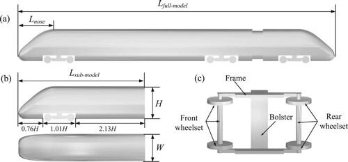
Figure 2. Computational domain of the full model and sub-model.

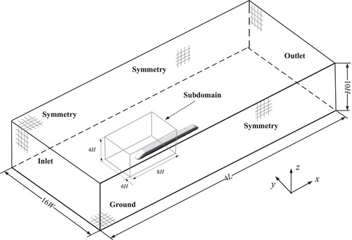
Table 2. Case descriptions.

Case	λ	U∞ (km/h)	Ma	St	Re
Case0	1/1	400	0.326	0.032f	2.7 × 10^7
Case1	1/10	400	0.326	0.0032f	2.7 × 10^6
Case2	1/10	40	0.0326	0.032f	2.7 × 10^5

Figure 3. Distribution of surface y+ values based on the full model of case0.

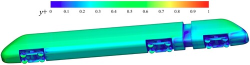
Figure 4. Position diagram of acoustic receivers (case0).

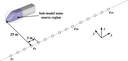
Figure 5. Comparison of acoustic results of train surface under different mesh densities.

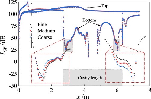
Figure 6. Distribution of grids on and around the train surface.

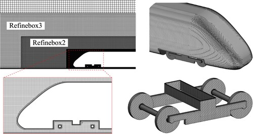
Table 3. Comparison of far-field noise results under different grid densities.

	Base		Grid
	size/m		number/million
	Full	Sub-	Full	Sub-	Max	Avg
Mesh	model	model	model	model	SPL/dB	SPL/dB
Fine	0.96	0.16	47.65	46.52	97.7	96.4
Medium		0.24		37.14	98.0	96.8
Coarse		0.32		29.47	98.5	97.3

Table 4. Solver settings for numerical simulation.

	Full-model	Sub-model
Simulation process	Steady simulation	Steady simulation	Unsteady simulation
Turbulent model	SST k-ω	SST k-ω	IDDES
Solver Type	Pressure-Based	Pressure-Based	Pressure-Based
Solution Methods	SIMPLE	SIMPLE	SIMPLE
Gradient	Least Squares Cell Based	Least Squares Cell Based	Least Squares Cell Based
Spatial Discretization	Second Order Upwind	Second Order Upwind	Bounded Central Differencing
Turbulent quantities	Second Order Upwind	Second Order Upwind	Second Order Upwind
Time Formulation	/	/	Second Order Implicit
Time step	/	/	CFL < 1

Figure 7. Isolated wheelset model for numerical validation.

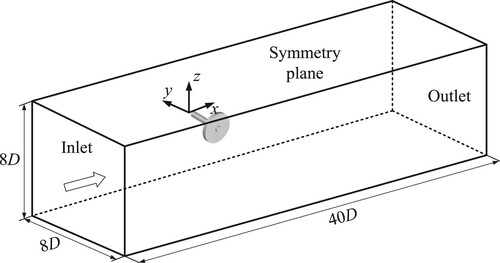
Figure 8. Comparison of noise spectra for far-field acoustic receivers: (a) top receiver and (b) side receiver.

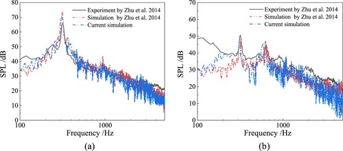
Figure 9. Time-averaged pressure distribution on the: (a) train surface and (b) train bottom.

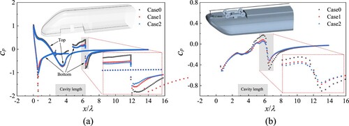
Figure 10. Train surface monitoring point location diagram.

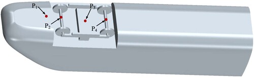
Figure 11. Spectrum characteristics of train surface pressure monitoring points: (a) Measurement points P₁–P₄ for case2, and (b) Measurement point P₂ for different cases.

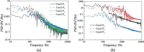
Figure 12. The instantaneous distribution of vortex structure in bogie region with different $\tilde{Q}$ values, coloured by velocity: (a) case0,(b) case1 and (c) case2.

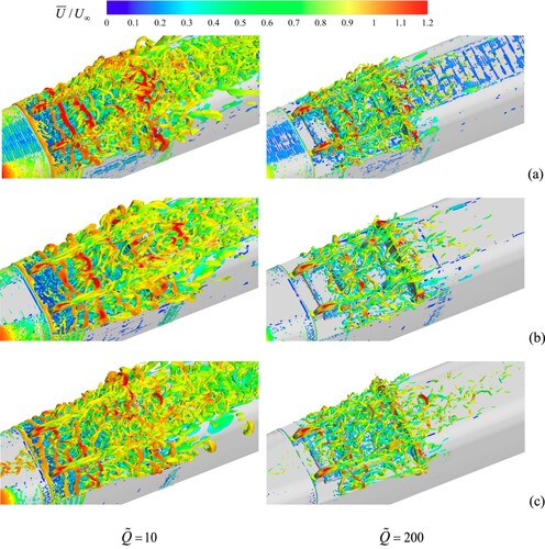
Figure 13. The instantaneous vorticity field distribution on the longitudinal central section (y = 0) and the vertical section (z = 0.18H): (a) case0, (b) case1 and (c) case2.

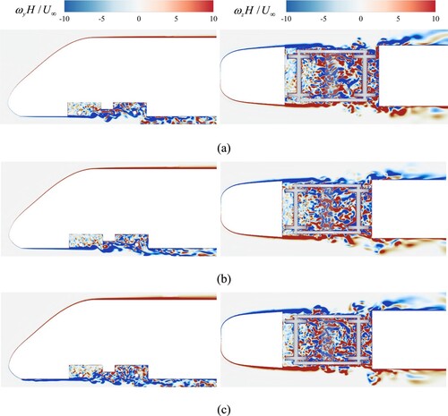
Figure 14. Comparison of flow field at the bottom of train: (a) dimensionless time-averaged velocity and (b) time-averaged vorticity magnitude.

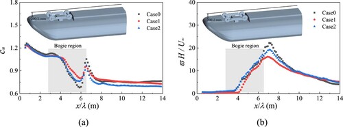
Figure 15. The instantaneous vortex core distribution in the bogie region: (a) case0, (b) case1 and (c) case2.

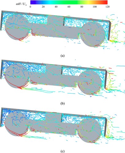
Figure 16. Surface pressure fluctuation distribution in the bogie region: (a) case0, (b) case1 and (c) case2.

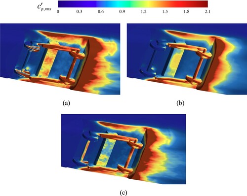
Figure 17. Mean velocity distribution near the wall of the bogie region: (a) case0, (b) case1 and (c) case2.

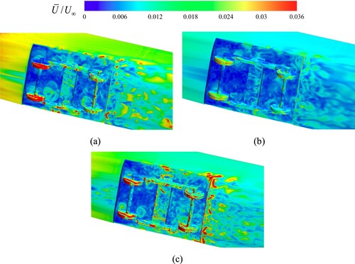
Figure 18. The instantaneous turbulent kinetic energy distribution around the train: (a) case0, (b) case1 and (c) case2.

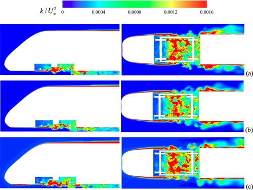
Figure 19. Division of sound source components.

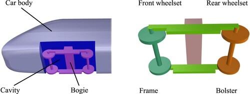
Figure 20. OASPL comparison of different components as noise sources: (a) case0, (b) case1 and (c) case2.

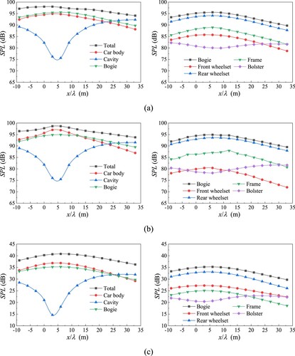
Figure 21. Comparison of OASPL results in different cases: (a) total, (b) car body, (c) cavity and (d) bogie.

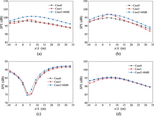
Figure 22. OASPL comparison for each component of the bogie: (a) front wheelset, (b) rear wheelset, (c) frame and (d) bolster.

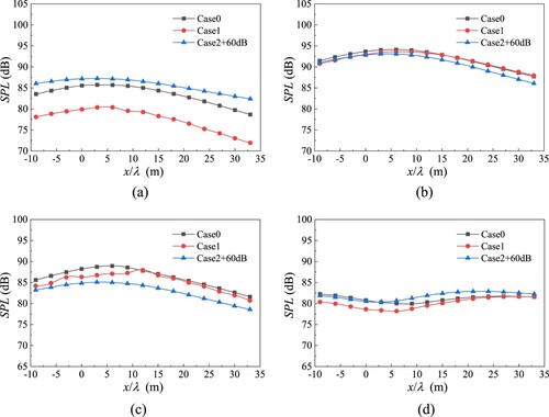
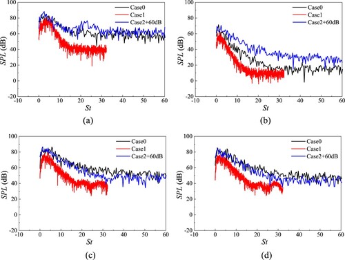
Figure 23. Comparison of noise spectra at receiver r₆, with a frequency resolution of 10 Hz: (a) car body, (b) cavity, (c) bogie and (d) rear wheelset.

Zhu, J. Y., Hu, Z. W., & Thompson, D. J. (2016). Flow behaviour and aeroacoustic characteristics of a simplified high-speed train bogie. Proceedings of the Institution of Mechanical Engineers Part F Journal of Rail and Rapid Transit, 230(7), 1642–1658. https://doi.org/10.1177/0954409715605129

 Web of Science ®Google Scholar

Zhu, J. Y., Hu, Z. W., & Thompson, D. J. (2018). The flow and flow-induced noise behaviour of a simplified high-speed train bogie in the cavity with and without a fairing. Proceedings of the Institution of Mechanical Engineers Part F Journal of Rail and Rapid Transit, 232(3), 759–773. https://doi.org/10.1177/0954409717691619

 Google Scholar

Minelli, G., Yao, H. D., Andersson, N., Höstmad, P., Forssén, J., & Krajnovic, S. (2020). An aeroacoustic study of the flow surrounding the front of a simplified ICE3 high-speed train model. Applied Acoustics, 160, 107125. https://doi.org/10.1016/j.apacoust.2019.107125

 Web of Science ®Google Scholar

Guo, Z., Liu, T., Xia, Y., & Liu, Z. (2022). Aerodynamic influence of the clearance under the cowcatcher of a high-speed train. Journal of Wind Engineering and Industrial Aerodynamics, 220, 104844. https://doi.org/10.1016/j.jweia.2021.104844

 Google Scholar

Shi, J. W., & Zhang, J. Y. (2024). Effect of bogie cavity endwall inclination on flow field and aerodynamic noise in the bogie region of high-speed trains. Computer Modeling in Engineering & Sciences, 139(2), 2175–2195. https://doi.org/10.32604/cmes.2023.043539

 Google Scholar

He, Y., Thompson, D., & Hu, Z. W. (2024). Aerodynamic noise from a high-speed train bogie with complex geometry under a leading car. Journal of Wind Engineering and Industrial Aerodynamics, 244, 105617. https://doi.org/10.1016/j.jweia.2023.105617

 Google Scholar

Data availability

The data that support the findings of this study are available from the corresponding author upon reasonable request.