A new implementation of FLEXPART with Enviro-HIRLAM meteorological input, and a case study during a heavy air pollution event

Figures & data

Figure 1. Workflow of enviro-HIRLAM+FLEXPART, IFS-ERA5+FLEXPART, and GFS-FNL+FLEXPART simulations we generated and compared in this study, including three models (enviro-HIRLAM, IFS and GFS), types of model runs, resolutions, output, steps of preprocessing, trajectory calculations and analysis, as well as types of meteorological input to FLEXPART. Inputs to enviro-HIRLAM, including initial and boundary conditions, and the data assimilation of observations are described in detail in section 2.2.3. Remark: ICs = initial conditions, BCs = boundary conditions, CAMS = Copernicus Atmosphere Monitoring Service, DA = data assimilation, EIs = emission inventories; EH0-EH3 = enviro-HIRLAM model meteorology. Colored arrows (green, cyan, blue, red) indicate enviro-HIRLAM meteorology as input for FLEXPART model corresponding nests (mother domain, nest 1, nest 2, nest 3).

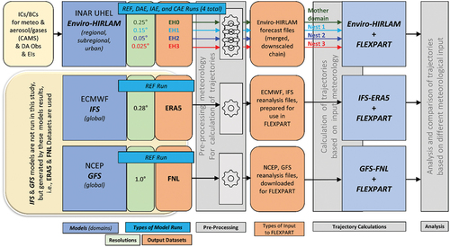
Figure 2. Map of the Enviro-HIRLAM nested model domains used in this study, with horizontal resolutions as follows, from largest to smallest: 0.25° (mother domain; green), 0.15° (cyan), 0.05° (blue), and 0.025° (red). The innermost nested domain is centered over the greater Beijing metropolitan area. Beijing is marked with the red cross.

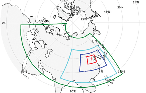
Figure 3. Visible satellite imagery of the north China plain, taken from the visible infrared imaging radiometer suite (VIIRS). Beijing is marked with the red cross. The images were captured shortly after noon local time on each day as the satellite passed overhead (i.e. 13 Nov. 04:38 UTC/12:38 LT; 14 Nov. 04:20 UTC/12:20 LT; 15 Nov. 04:03 UTC/12:03 LT; 16 Nov. 05:22 UTC/13:22 LT).

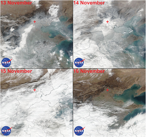
Figure 4. Time-series of meteorology (air temperature, relative humidity, atmospheric pressure, precipitation, visibility, wind speed and direction) and PM_2.5 concentration from 12 UTC 14 November (T1) through 12 UTC 15 November 2018 (T5), observed at the BUCT-AHL station in Beijing, China.

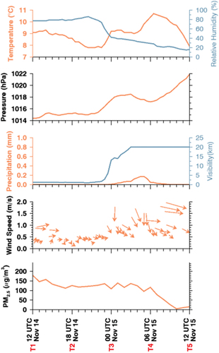
Figure 5. Spatiotemporal positions of atmospheric backward trajectories calculated by FLEXPART using different meteorological inputs (from model runs: IFS-ERA5 (extracted at 0.25° horizontal resolution), GFS-FNL, and enviro-HIRLAM (EH), with full downscaling chain, without aerosol effects (REF) and with aerosol effects (CAE)) arriving at the BUCT-AHL measurement station at height 500 m above ground level with arrival times of a.) T1; b.) T2; c.) T3; d.) T4; and e.) T5. In addition to the center point over the station, an ensemble representing a 20 km × 20 km box (described in Section 2.1.3) is plotted in lighter colors, with the four corners (northeast, northwest, southeast, and southwest). Vertical profiles of trajectories, as a function of altitude (km) vs. distance (km) to the station along trajectories, are also plotted above each subplot map, together with the underlying terrain. The numbers on the trajectories indicate the time (in days) before arrival at the station.

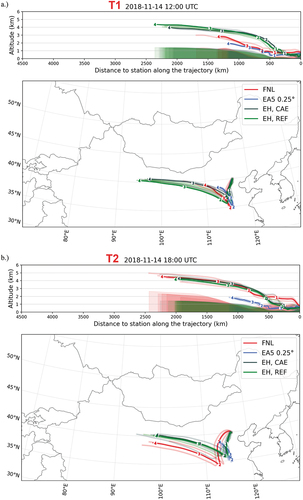
Figure 5. (Continued).

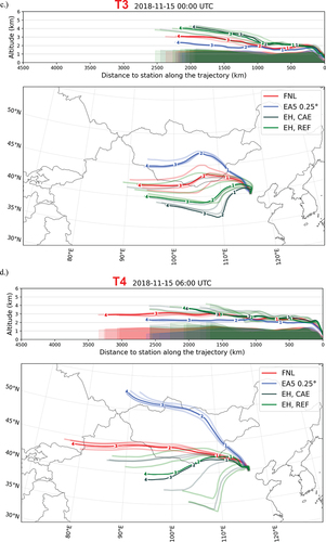
Figure 6. Differences in atmospheric trajectories. Each colored line represents the difference between two trajectories, arriving at the same time but calculated using different meteorology. The six panels compare all three FLEXPART realizations (input from ERA5, FNL, or enviro-HIRLAM with combined aerosol effects (CAE)) with each other. The label on the right shows the reference trajectory; the axis on the left shows the distance from comparison trajectory to reference trajectory (panel a.) or relative difference, defined as distance to station (along trajectory) versus distance to reference trajectory (panel b.) solid black lines show the average for 14 November (during the haze episode) and dashed black lines show the average for 15 November (after the haze has cleared out).

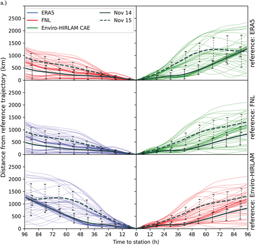
Figure 6. (Continued).

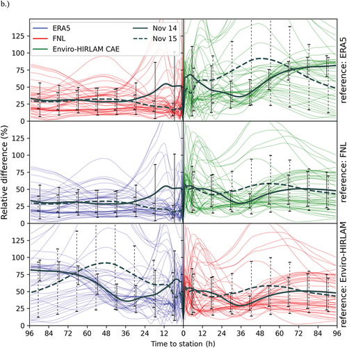
Figure 7. FLEXPART trajectories calculated based on enviro-HIRLAM meteorology with combined aerosol effects (CAE), direct aerosol effects (DAE), indirect aerosol effects (IAE), and control/reference (REF) without aerosol effects included. Arrival times are as follows: a.) T1; b.) T2; c.) T3; d.) T4; and e.) T5. The numbers on the trajectories indicate time (in days) before arrival at the station.

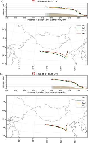
Figure 7. (Continued).

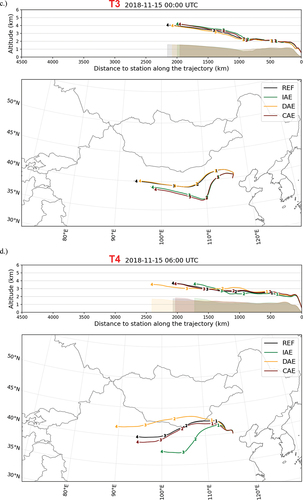
Figure 7. (Continued).

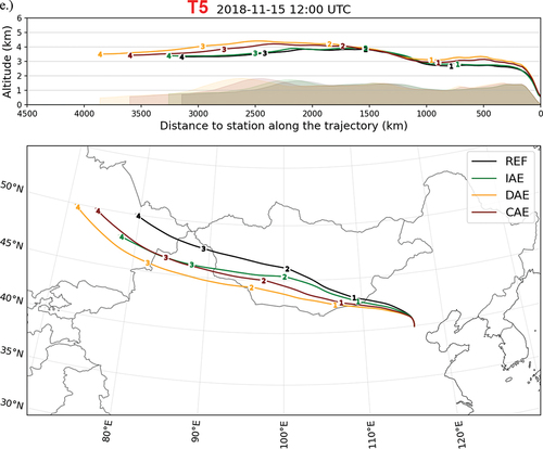
Figure 8. Spatiotemporal distribution of dispersion of particles (modelled by FLEXPART using GFS-FNL, IFS-ERA5, and enviro-HIRLAM CAE meteorological inputs), calculated as emission sensitivity (in units of seconds), arriving at the BUCT-AHL measurement station with arrival times at: a.) T1; b.) T2; c.) T3; d.) T4; and e.) T5. The emission sensitivity is related to the residence time of dispersed particles in the atmosphere, and it gives an idea of the source area of potential emissions of pollutants that could eventually arrive at the station.

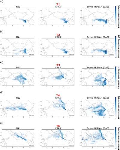
Figure 5. (Continued).

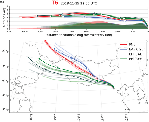
Table 1. Percent of emission sensitivity values calculated by FLEXPART (based on meteorology from 3 different models, including Enviro-HIRLAM model output for 4 aerosol modes), divided into quadrants (NW, NE, SW, and SE) around the BUCT-AHL station. Darker shading represents higher values.

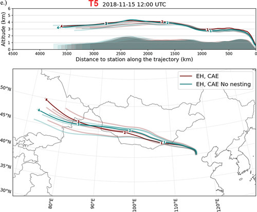
Figure 9. Atmospheric trajectories calculated by FLEXPART without nesting (based on enviro-HIRLAM CAE meteorology at 0.25° horizontal resolution) and fully nested (i.e. mother domain with all three higher-resolution nests & based on enviro-HIRLAM-CAE meteorology at 0.25°, 0.15°, 0.05° and 0.025° horizontal resolutions, respectively) at arrival times at: a.) T2; b.) T2; c.) T3; d.) T4; and e.) T5. The numbers on the trajectories indicate time (in days) before arrival at the station.

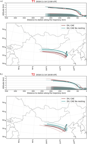
Figure 9. (Continued).

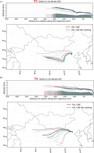
Figure 9. (Continued).

Data availability statement

1. New FLEXPART code

The FLEXPART code used for this publication has been uploaded to Zenodo, available at https://doi.org/10.5281/zenodo.8300429. The code will also be available in a repository on the FLEXPART website at https://doi.org/10.5281/zenodo.8300429, and new versions will be published here. We suggest potential users who wish to use the Enviro-HIRLAM-FLEXPART modelling system use the version that will be published on the FLEXPART website. We also plan to work with the FLEXPART team to integrate this into a future version of the public FLEXPART version. We suggest that users refer to the official FLEXPART website for the latest version.

2. Enviro-HIRLAM post-processing script

An example script to select and merge the Enviro-HIRLAM output for use in FLEXPART is in Appendix C of this manuscript.

3. Enviro-HIRLAM model code

The Enviro-HIRLAM modelling system is a community model. The source code is available for non-commercial use (i.e. research, development and science education) upon agreement through contact with Alexander Mahura ([email protected]), Bent Sass ([email protected]) and Roman Nuterman ([email protected]). Documentation, educational materials and practical exercises are available from http://hirlam.org and hirlam.org/index.php/documentation/chemistry-branch, and Young Scientist Schools (netfam.fmi.fi/YSSS08, www.ysss.osenu.org.ua; aveirosummerschool2014.web.ua.pt and https://megapolis2021.ru).