Figures & data
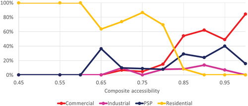
Figure 1. Location of Delhi Metropolitan area in the National Capital Region of India.
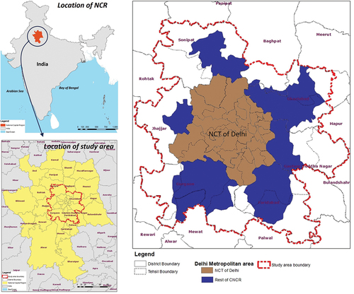
Figure 2. Transport network (nodes and links) in the study area.
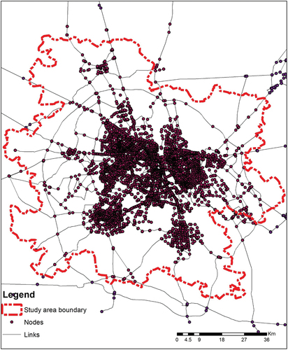
Figure 3. Framework to assess path evaluation function and centrality measures.
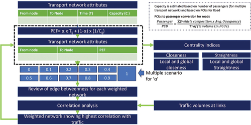
Figure 4. Transport network characteristics for the study area. a) represents the typology of transport network in the study area; b) represents the peak hour speeds on the identified transport network i.E roads and Metro system.
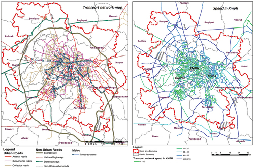
Table 1. Transport network characteristics in the study area.
Figure 5. Existing landuse distribution for the study area-2021.
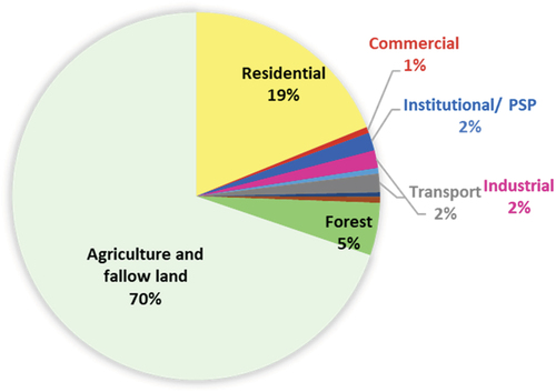
Figure 6. Existing landuse of the study area-2021.
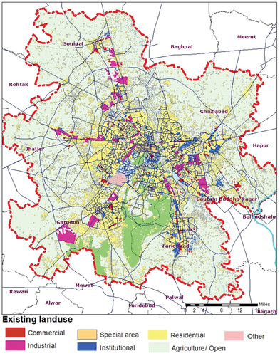
Figure 7. Correlation assessment for varying betweenness centrality (with varying path evaluation function (PEF)) and traffic flow.
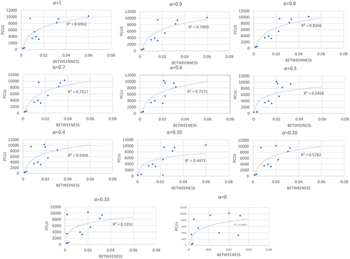
Figure 8. Correlation coefficients for separate α values.
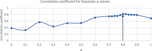
Figure 9. Centrality maps for the study area; a) shows global closeness centrality, b) shows local closeness centrality, c)shows global straightness centrality and d) local straightness centrality for the study area.
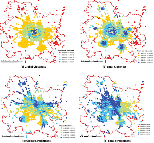
Figure 10. Results of multinomial logistics regression for various centrality measures and landuse (here this represents direction of relationship with respect to commercial); landuse 1 is residential, landuse 2 is industrial and landuse 3 is PSP/institutional.
Figure 11. Composite centrality.
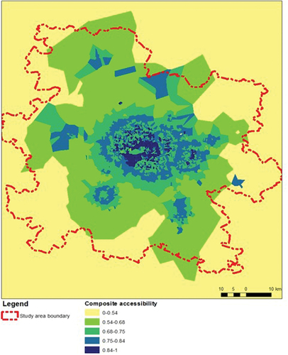
Figure 12. Relationship between composite centrality and landuse.
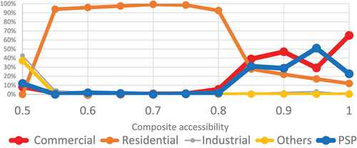
Table 2. Key landuse across centrality ranges along urban roads.
Figure 13. Relationship between composite centrality and landuse along: a) arterial roads, b) Sub arterial roads and c) Collector roads.
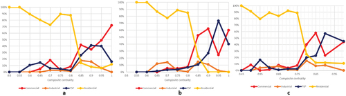
Figure 14. Relationship between composite centrality and landuse along non-urban/interurban highways.
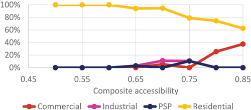
Figure 15. Relationship between composite centrality and landuse along Metro system.