
Figures & data
Figure 1. (a) Particle size distribution of calcined clay-1 (CC-1), calcined clay-2 (CC-2), Portland cement, limestone powder, and gypsum; (b) X-ray diffraction (Cu-Kα radiation) patterns of CC-1, CC-2, Portland cement, and limestone powder. Cal-calcite, Gp-gypsum, C3S-alite, C3A-tricalcium aluminate, Mul-mullite, Qz-quartz, Kln-kaolinite.
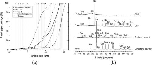
Table 1. Oxide compositions of binding materials.
Table 2. Physical characteristics of all dry components used in this study.
Table 3. Mix designs of cementitious materials (unit: kg/m3).
Figure 2. Illustration of the rheometer used in this study. (a) Photograph of Anton Paar MCR 302e rheometer; (b) Photograph of the four-blade vane and the cylindrical measuring cell.
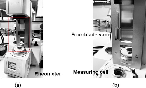
Figure 3. Illustration of the flow curve test. (a) Flow curve test protocol used in the study; (b) A typical plot of flow curve; (c) The average shear stresses with different shear rates. The descending curve was fitted using the modified Bingham model.
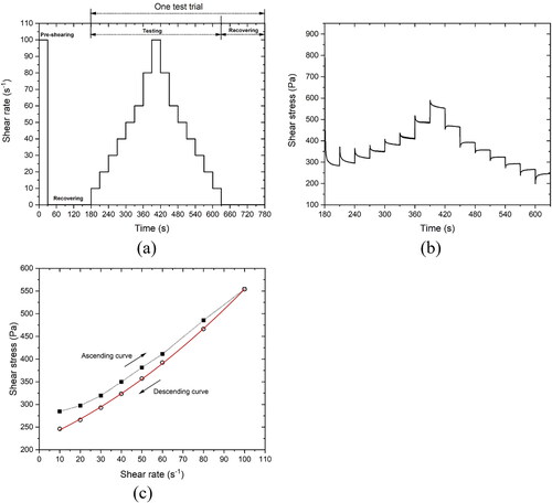
Figure 4. A typical curve of constant shear rate test.
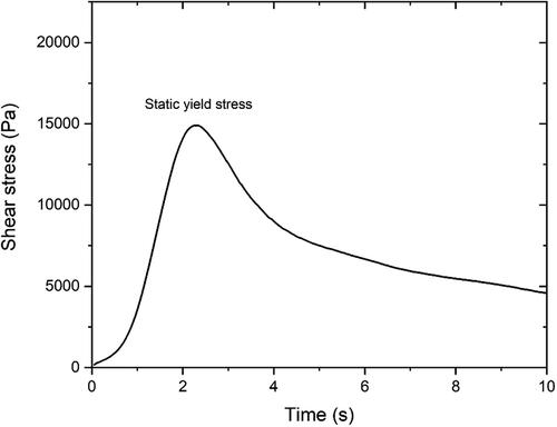
Figure 5. Illustration of applied sinusoidal strain and measured shear stress
for a typical viscoelastic material in SAOS-time sweep test.
is defined as phase/loss angle. Loss factor = tan(
) = G''/G'. Adapted from [Citation49].
![Figure 5. Illustration of applied sinusoidal strain γ(t) and measured shear stress τ(t) for a typical viscoelastic material in SAOS-time sweep test. δ is defined as phase/loss angle. Loss factor = tan(δ) = G''/G'. Adapted from [Citation49].](/cms/asset/8bf9d28f-abe5-4b64-9bb3-cb46af9a3b3c/tscm_a_2169965_f0005_b.jpg)
Figure 6. Flow curves at the material ages of 10 min, 20 min, and 30 min – descending curves fitted by the modified Bingham model of (a) mixtures B45, M45, and H45, (b) mixtures B45 and B45-1; (c) Dynamic yield stress of various mixtures.
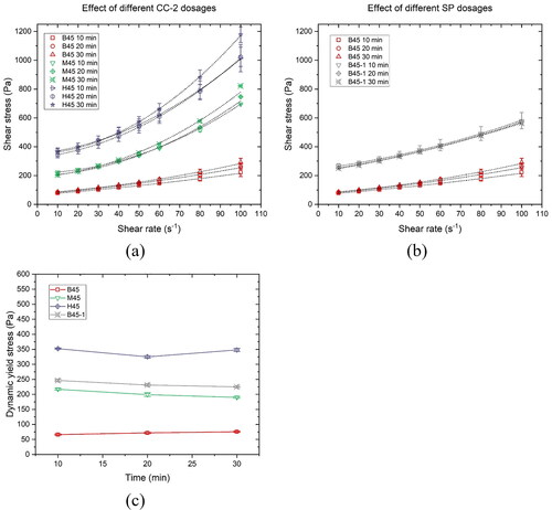
Table 4. Rheological characteristics of different mixtures fitted by the modified Bingham model.
Figure 7. Constant shear rate-single sample test results of (a) mixture B45, (b) mixture B60, (c) mixture B75, (d) mixture M45, (e) mixture H45, (f) mixture 45-1.
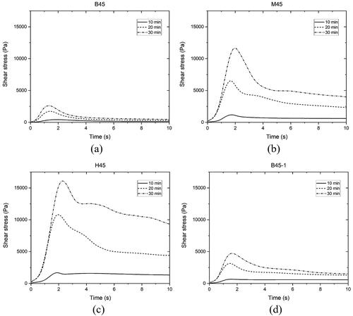
Figure 8. Comparison of static yield stress evolution and structuration rate between mixtures. (a) Static yield stress evolution of different mixtures within the first 30 min; (b) Structuration rate Athix of different mixtures obtained by linear fitting.
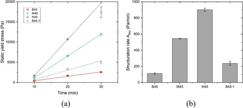
Figure 9. Amplitude sweep test results at 8 min: the critical strain for different mixtures is about 0.1% at the angular frequency of 1 Hz.
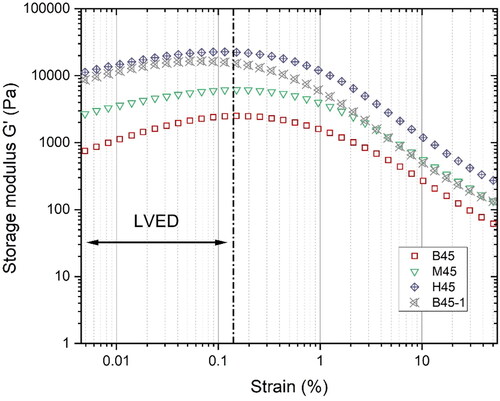
Figure 10. SAOS-time sweep test results of different mixtures from 22 min to 72 min: (a) Storage modulus G' development with time – linear scale; (b) Storage modulus G' development with time – logarithmic scale; (c) Loss modulus G'' development with time; (d) Loss factor development with time.
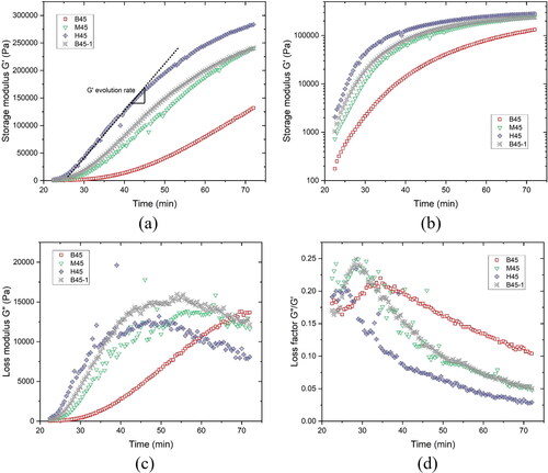
Figure 11. Comparison of peak time of loss factor and G' evolution rate between mixtures. (a) The peak time of loss factor; (b) G' evolution rate of different mixtures.
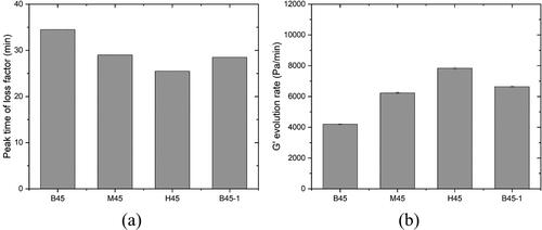
Figure 12. Isothermal calorimetry test results: (a) Normalized heat flow by mass of paste with time (48 h); (b) Normalized cumulative heat by mass of paste with time (168 h); (c) The required time to the C3S hydration peak of different mixtures; (d) The slope of the acceleration period of different mixtures.
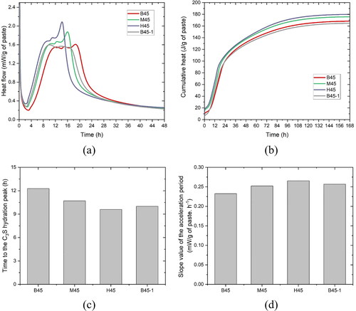
Table 5. Solid volume fraction, total specific surface area, water film thickness and mean interparticle distance of different mixtures.
Figure 13. Comparison of maximum packing density, mean interparticle distance and water film thickness between mixtures. (a) The maximum packing density of studied mixtures; (b) Correlation between mean interparticle distance and water film thickness.
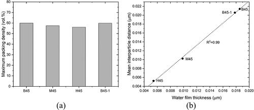
Figure 14. The relationship between rheological indicators measured using rheometry and mean interparticle distance. (a) Correlation between dynamic yield stress fitted by the modified Bingham model (at 10 min, 20 min, and 30 min) and mean interparticle distance; (b) Correlation between static yield stress obtained by CSR test (at 10 min, 20 min, and 30 min) and mean interparticle distance; (c) Correlation between structuration rate Athix (10–30 min) and mean interparticle distance; (d) Correlation between G' evolution rate from SAOS-time sweep test and mean interparticle distance.
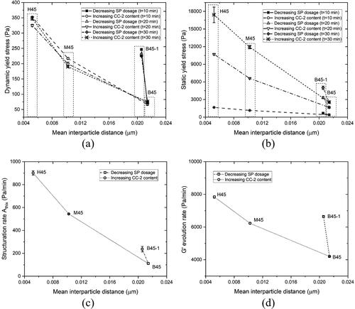
Figure A1. ESEM-EDS elemental mapping analysis of 28-day B45 sample; (a) BSE micrograph; (b) Elemental mapping image of Ca (calcium); (c) Elemental mapping image of Si (silicon); (d) Elemental mapping image of Al (aluminum); (e) Overlay masks of quartz (Cyan) and metakaolin (Yellow) particles determined using Compass + XPhase on Pathfinder X-ray Microanalysis Software (Thermo Fisher Scientific).
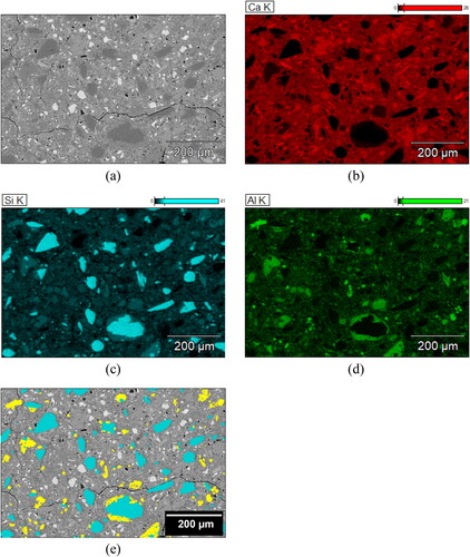
Table A1. Rheological characteristics of different mixtures fitted by the Herschel-Bulkley model.