Percolation and Universal Scaling in Composite Infiltration Processing

Figures & data

Figure 1. Different views of pressure infiltration. (a) Sketch of metal matrix composite pressure infiltration. (b) In conventional modeling, the process is simulated by integrating local flow laws over a representative volume element (RVE), which is then used as a differential element in a continuum-based simulation of the process across the composite part to be produced. (c) Infiltration as governed by percolation: the metal structure is fractal, invalidating the RVE approach.

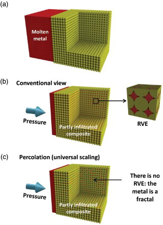
Figure 2. Fully infiltrated samples. (a) Microstructure in each composite investigated here after full infiltration (S=1). (b) Measured drainage curves for each system.

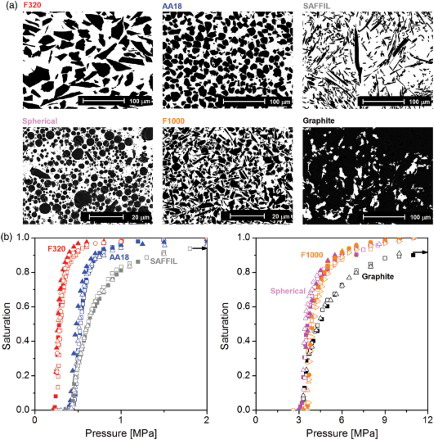
Figure 3. Partially infiltrated samples. (a) Low-magnification (left) and high-magnification (right) view of the microstructure of each composite system, taken at low saturation (S<0.5). (b) Measured drainage curves for each system, plotted to test Equation (1). Average sample saturation for both lower and higher magnification micrographs is 0.1 for Saffil^™ short fibers, 0.2 for all other systems.

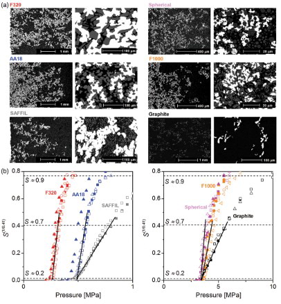
Table 1. Solid preforms explored in this work (nature, volume fraction solid and density of the solid) together with measured infiltration characteristics (approximate value of the pressure P_max required to fully infiltrate the preform, constants P_c and C in the scaling law describing initial stages of infiltration, Equation (3); constants λ and P_b of the Brooks and Corey relation, Equation (1)).

	Volume fraction, Vr	Bulk density (g/cm^3)	Pmax (S=1) (MPa)	Pc (0.6 ≥S≥0.2)	Constant C (MPa^−β)	λ (0.9 ≥S≥0.6)	Pb (0.9 ≥S≥0.6)
F320	0.44±0.02	4.0	5	0.25±0.01	2.16±0.17	4.0±0.6	0.23±0.02
AA18	0.54±0.02	4.0	5	0.47±0.02	1.78±0.09	5.0±0.3	0.44±0.02
SAFFIL	0.30±0.01	3.5	8	0.47±0.01	1.08±0.02	2.0±0.1	0.43±0.02
Spherical	0.73±0.02	3.9	10	3.31±0.05	0.89±0.13	3.3±0.6	2.79±0.25
F1000	0.54±0.03	3.9	11	3.52±0.10	0.79±0.03	3.8±0.5	3.15±0.14
Graphite	0.80±0.01	2.3	17	3.38±0.02	0.51±0.02	2.1±0.1	3.09±0.14

Figure 4. Measuring the metal fractal dimension in partly infiltrated composites. (a) Backscattered scanning electron image of a partially infiltrated composite (AA18/Cu at P=0.46 MPa). The colored squares (768×768 pixels) indicate the area used to measure the fractal dimension using the box counting method (‘ImageJ’ function: ‘Fractal box counter’, size of the boxes: 2, 3, 4, 6, 8, 12, 16, 24, 32, 48, 64, 96, 128 and 192 pixels) and the corresponding thresholded images (in which the metal is turned black and the rest white). (b and c): evolution of the measured two-dimensional fractal dimension D_2D computed from the average slope through the range of data (b), showing (c) that it tends to increase somewhat with increasing metal volume fraction V_m (which in turn increases from the preform center to its outer surface in contact with the metal bath); (d): range of variation of D_2D with corresponding range for V_m, and final estimated value of D=(D_2D+1), the 3-D fractal dimension of the metal cluster in the most porous (central preform) region for each of the composite systems investigated.

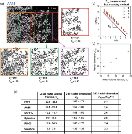
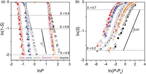
Figure 5. Confrontation of data with Equations (1) and (3) using logarithmic coordinates. Measured drainage curves for all systems explored here (Figure 2(b)) replotted in logarithmic coordinates to test (a) Equation (3), and (b) Equation (1) (using values of P_c obtained by extrapolation of a linear regression of S^(1/0.41) over the range 0.02≤S^(1/0.41)≤0.35, corresponding to 0.2≤S≤0.65). Note that portions of the curves in these log-log coordinates are affected in (a) near S=1 by uncertainty in the pore volume (hence data are only plotted up to S=0.9) and in (b) near S=0 by uncertainty in P_c (this does not affect the comparison if data are plotted as in Figure 3(b)).