Figures & data
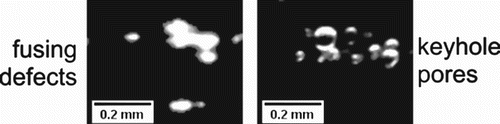
Figure 1. Porosity as a measure for the total number of defects measured by microscopy (2D), tomography (3D), and the Archimedes method as a function of the energy density applied during SLM. ‘sample 1’ and ‘sample 2’ indicate the conditions chosen for the further investigation by x-ray refraction radiography.
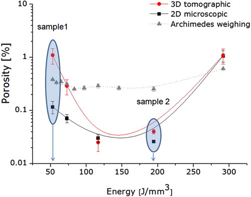
Figure 2. Tomographic (3D) (a,b) and microscopic (2D) (c,d) depictions of the defects observed in the SLM produced Ti64 parts: for sample 1 (a,c) and sample 2 (b,d). The bounding cylinders (a,b) have a size of 800 µm diameter and 700 µm height, the Ti64 alloy is transparent.
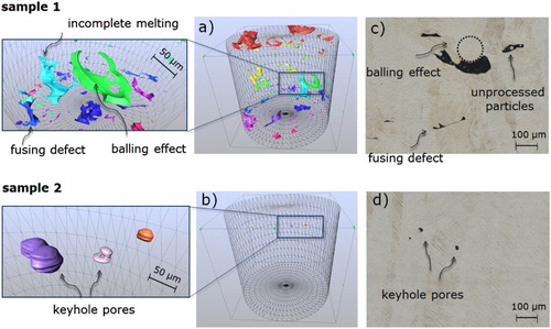
Figure 3. Sketch of the experimental setup ‘ABI’ for X-ray refraction radiography at BAMline.
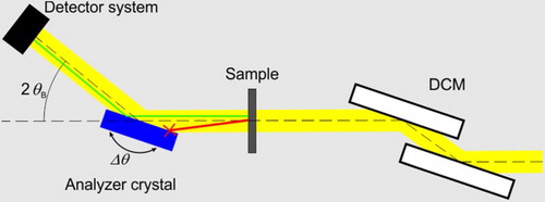
Figure 4. (Left) 2D distribution of the specific surface in mm−1 of sample 1 (a) and sample 2 (b) from SXRR; (right) 2D distribution of porosity in % of sample 1 (c) and sample 2 (d) from conventional radiography.
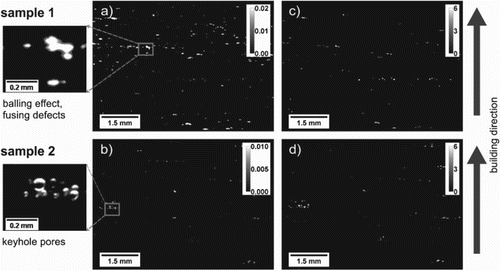
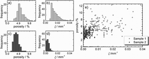
Figure 5. Histograms of the average specific surface and average porosity of the segmented defects in sample 1 (a, b) and sample 2 (c, d); scatter plot of average porosity vs. average specific surface for each defect (e).