Achieving fully-equiaxed fine β-grains in titanium alloy produced by additive manufacturing

Figures & data

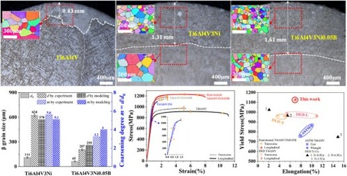
Table 1. Processing parameters for DED.

Laser power (kW)	Scanning velocity (mm/min)	Powder feed rate (kg/h)	Nominal increment (mm)	Spot diameter (mm)
2	900	0.5	0.15	5

Figure 1. The β-grains at the top of Ti6Al4VxNiyB and the initial solidification mechanism of the last layer. (a), (d) Ti6Al4V; (b), (e) Ti6Al4V3Ni; (c), (f) Ti6Al4V3Ni0.05B; (g) grain size d₀ plotted against the inverse Q. (The dashed white lines in a-c separate the equiaxed grains obtained only by solidification from the ones subjected to subsequent thermal-cycling. T_E is the equilibrium liquidus temperature and ΔT_n is the critical undercooling for nucleation).

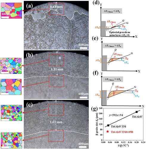
Table 2. The Q, ΔT₀, m_l, k and Q_i.

Alloy	Q	ΔT0 (K)	Element	ml (K/wt%)	k	Qi
Ti6Al4V	5.1	5.4	Al	5.64	1.15	5.08
			V	0.42	1.01	0.02
Ti6Al4V3Ni	34.02	111.8	Al	6.26	1.09	3.38
			V	0.66	1.0	0
			Ni	−13.80	0.26	30.64
Ti6Al4V3Ni0.05B	39.05	188.7	Al	6.28	1.10	3.77
			V	0.68	0.99	−0.03
			Ni	−13.94	0.26	30.95
			B	−88.70	0.016	4.36

Figure 2. The β-grains at the middle of the Ti6Al4V3NiyB deposits. (a) Ti6Al4V3Ni, (b) Ti6Al4V3Ni0.05B; (c) β-grain size and coarsening degree m; (d) the function of the simulated m with regard to d₀, and the symbols represent the experimental value; the simulated δd_i, d = d₀+Σδd_i, δM_i and M = ΣδM_i with regard to the thermal-cycling number (T_β˂T_p˂T_s) in (e) Ti6Al4V3Ni and (f) Ti6Al4V3Ni0.05B. (T_s and T_β are calculated using Thermo-Calc.).

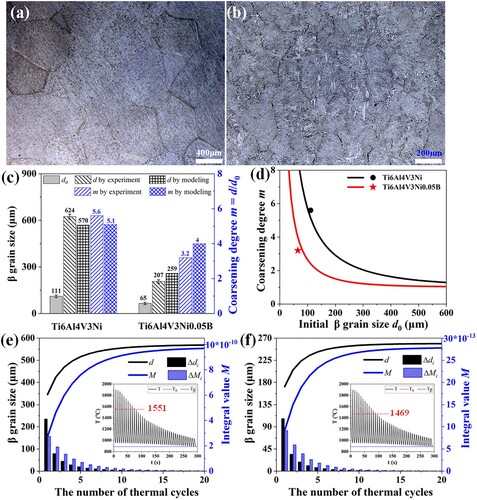
Figure 3. The microstructures at the middle of the Ti6Al4VxNiyB deposits. As-built: (a) Ti6Al4V, (b) Ti6Al4V3Ni, and (c) Ti6Al4V3Ni0.05B, (d) heat-treated Ti6Al4V3Ni0.05B.

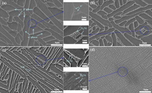
Figure 4. Mechanical properties of Ti6Al4VxNiyB alloys. (a) Representative engineering stress–strain curves; the error bars (UTS and EL) represent one standard deviation. (b) Tensile properties for heat-treated Ti6Al4V3Ni0.05B are comparable with Ti-Cu [6] and Ti6Al4V [10] by DED and the ASTM standard for Ti6Al4V [32]. (c) Anisotropy (the calculation method is shown in [21]).

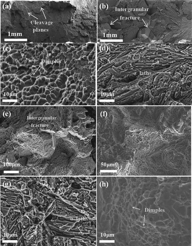
Figure 5. Fracture surfaces of longitudinal specimens: (a) (c) as-built Ti6Al4V, (b) (d) as-built Ti6Al4V3Ni, Ti6Al4V3Ni0.05B (e) (f) as-built and (g) (h) heat-treated.

Zhang D, Qiu D, Gibson MA, et al. Additive manufacturing of ultrafine-grained high-strength titanium alloys. Nature. 2019;576:91–95.

 PubMed Web of Science ®Google Scholar

Kok Y, Tan XP, Wang P, et al. Anisotropy and heterogeneity of microstructure and mechanical properties in metal additive manufacturing: a critical review. Mater Des. 2018;139:565–586.

 Web of Science ®Google Scholar

Zhang D, Sun S, Qiu D, et al. Metal alloys for fusion-based additive manufacturing. Adv Eng Mater. 2018;20:1700952.

 Web of Science ®Google Scholar

Xue A, Lin X, Wang L, et al. Influence of trace boron addition on microstructure, tensile properties and their anisotropy of Ti6Al4V fabricated by laser directed energy deposition. Mater Des. 2019;181:107943.

 Web of Science ®Google Scholar