Breaking hardness and electrical conductivity trade-off in Cu-Ti alloys through machine learning and Pareto front

Figures & data

Figure 1. Correlation between cold rolling deformation, aging time, solution temperature, and the properties for pure components ((a)–(c)), and Cu-Ti alloys ((d)–(f), (g)–(i), and (j)–(l)).

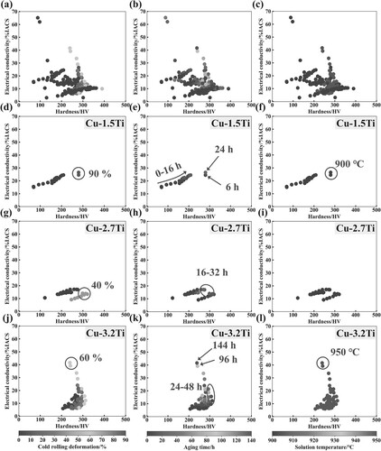
Figure 2. (a) Three newly expected data (five-pointed stars) designed by the Pareto front technique; (b) a comparison between the experimental properties of the designed alloys and those from the literature reports [8,20–24]; (c) and (d) represent the experimental hardness and electrical conductivity at different stages for the three designed alloys; (e) Cu-Ti Phase diagram (Ti < 10wt.%) [29]; (f) Simulated mean radius of precipitates, compared with the experimental data.

Table 1. List of compositions and process parameters of three selected alloys.

	Compositions		Process parameters						Predicted properties
No.	Cu/wt.%	Ti/wt.%	CRD/%	STT/^oC	ST/h	ATT/^oC	AT/h	H2/MPa	MH/HV	EC/%IACS
1#	Bal.	2	60	900	2.25	380	24	0	282.6	22.4
2#	Bal.	2.2	60	900	1	380	24	0	363.8	19.5
3#	Bal.	3.5	60	900	1	380	24	0	408.4	16.9

Figure 3. Measured microstructures of designed alloys: (a) STEM-HAADF image of the precipitates in Alloy 2# aged at 380°C for 48 h. (b) and (c) depict the elemental mappings for Cu and Ti, respectively, from the area shown in (a). Figures (e) and (f) respectively depict the magnified micrograph and FFT image of Area 1 in (d), while (g) and (h) correspond to Area 2;(i) the positions of β’-Cu₄Ti tetragonal lattice diffraction spots along the [001]_Cu axis [34]; (j) shows the morphologies and average sizes of precipitates in Alloy 2# aged for 24 h; (k) for Alloy 1# aged for 48 h; (l) for Alloy 2# aged for 48 h; (m) for Alloy 3# aged for 48 h.

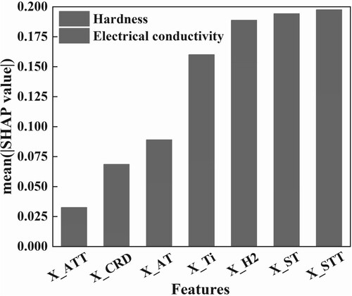
Figure 4. Influence of each input variable on model predictions (SHAP value). The blue signifies contribution to electrical conductivity, while the red indicates contribution to hardness. The length of the bar corresponds to the strength of the effect.

Nagarjuna S, Balasubramanian K, Sarma DS. Effect of prior cold work on mechanical properties, electrical conductivity and microstructure of aged Cu-Ti alloys. J Mater Sci. 1999;34(12):2929–2942. doi:10.1023/A:1004603906359

 Web of Science ®Google Scholar

Yang H, Zeng B, Wang H, et al. Phase equilibria and thermodynamic re-assessment of the Cu–Ti system. Calphad. 2023;82:102594. doi:10.1016/j.calphad.2023.102594

 Web of Science ®Google Scholar

Rouxel B, Cayron C, Bornand J, et al. Micro-addition of Fe in highly alloyed Cu-Ti alloys to improve both formability and strength. Mater Des. 2022;213:110340. doi:10.1016/j.matdes.2021.110340

 Web of Science ®Google Scholar