Figures & data
Table 1. Computational settings of high-resolution typhoon model (HTM)
Figure 1. Computational domain for the high-resolution typhoon model (HTM) with the sample track of Typhoon CHABA (2004). Black, blue, and green squares are D1, D2, and D3 domains, respectively. The figures on the top right show the horizontal distributions of Pc calculated in D2 and D3 (contoured at every 20 hPa). The figures on the bottom right show the horizontal distributions of wind speed at a 10 m height calculated in D2 and D3 (contoured at every 10 m/s).
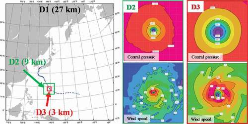
Figure 2. Computational flow for the pseudo-global warming downscaling experiment (PGWD) method. The left, middle, and right columns show the flows of the present-climate experiment, future-climate experiment, and horizontal resolution at each calculation step, respectively.
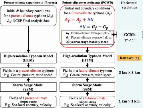
Figure 3. Observed tracks of target typhoons from genesis to decay, according to the JMA best track.
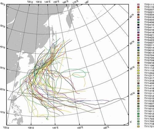
Table 2. List of general circulation models (GCMs) used for pseudo-global warming downscaling experiments (PGWDs). The (a) historical and (b) RCP8.5 data were obtained from 15 and 8 GCMs, respectively, in the Coupled Model Intercomparison Project 5 (CMIP5) (IPCC, Citation2013). These GCMs shown in table (a) are used for creating that data period of 2000–2005 from the historical of CMIP5, the GCMs in table (b) are used for creating that data period of 2006–2019 and 2080–2099. Global warming difference in present-climate is created by weighted averaging according to the length of the data periods (6 years for historical GCMs and 14 years for future GCMs)
Figure 4. Differences in the time periods covered by GCMs in CMIP5 and PGWDs in this study, and their respective definitions of “present climate” and “future climate” (modified from Figure SPM. 7 in IPCC AR5 WG1 (Intergovernmental Panel on Climate Change, Fifth Assessment Report, Working Group I. 2013. “Summary for policymakers.” in Climate Change 2013: The Physical Science Basis, edited by the Intergovernmental Panel on Climate Change. https://www.ipcc.ch/report/ar5/wg1/summary-for-policymakers/). This study defines 2000–2019 as the present climate and 2080–2099 as the future climate. As the defined period of this study is different from that of CMIP5 GCMs, it is adjusted when calculating the global warming difference (IPCC, Citation2013b).
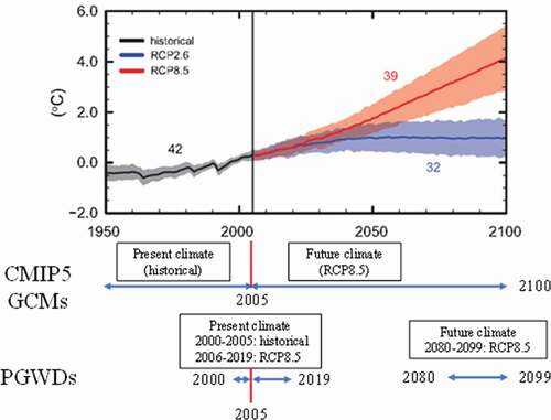
Figure 5. Distribution for continuity among GCM data used in this study. Ensemble mean distribution of temperature at 300 hPa for (a) 2000–2005 and (b) 2006–2019. The contours are drawn every 2.5 K. Ensemble mean distribution of SST for (c) 2000–2005 and (d) 2006–2019. The contours are drawn every 2.5 K. Differences in ensemble mean of (e) air temperature at 300 hPa and (f) SST from 15 GCMs in 2000–2005 and 8 GCMs in 2006–2019. The contours are drawn every 1.0 K (air temperature) and 0.5 K (SST).
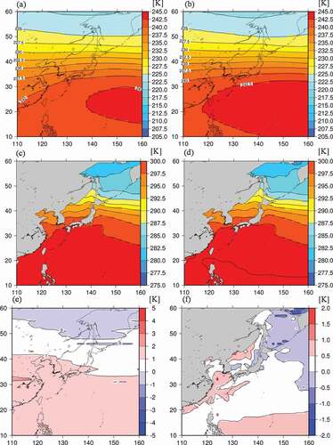
Figure 6. Scatter diagrams of central pressure (Pc) at (a) peak and (b) landfall times for observed (JMA best track) and estimated (HTM) typhoons.
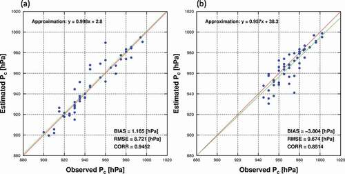
Figure 7. Scatter diagram of the radius of the maximum wind speed (Rm) at landfall time for observed (Myers Citation1954) and estimated (HTM) typhoons.
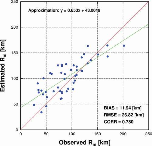
Figure 8. Relative frequency distributions of central pressure (Pc) at peak times for target typhoons in observations (JMA best track: dark blue bars), present-climate experiments (HTM: blue bars), and future-climate experiments (HTM: Orange bars). Average indicates the average value for each distribution.
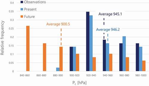
Figure 9. Relative frequency distributions of central pressure (Pc) at landfall times for target typhoons in observations (JMA best track: dark blue), present-climate experiments (HTM: blue bars), and future-climate experiments (HTM: Orange bars). Average indicates the average value for each distribution.
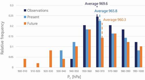
Figure 10. Scatter plot of Pc between present and future climates: (a) Pc at the peak times and (b) Pc at the landfall times – the horizontal axis represents the Pc in the present climate, and the vertical axis represents the Pc in the future climate. The blue line shows the regression line and the green line shows y = x.
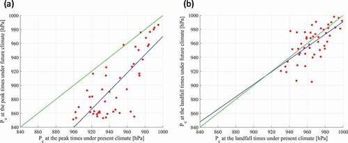
Figure 11. Horizontal distribution of (Upper) minimum central pressure by MPI theory (Bister and Emanuel Citation2002), (Middle) sea surface temperature (SST), and (Lower) absolute degree of vertical wind shear at 300–850 hPa. (a) is the distribution under the present climate (2000–2019), (b) is the distribution under the future climate (2080–2099), and (c) is the distribution of future changes [(b) future − (a) present]. Each value used the frequency-weighted averaged value obtained using the number of typhoons in each month, derived from CMIP5 GCMs.
![Figure 11. Horizontal distribution of (Upper) minimum central pressure by MPI theory (Bister and Emanuel Citation2002), (Middle) sea surface temperature (SST), and (Lower) absolute degree of vertical wind shear at 300–850 hPa. (a) is the distribution under the present climate (2000–2019), (b) is the distribution under the future climate (2080–2099), and (c) is the distribution of future changes [(b) future − (a) present]. Each value used the frequency-weighted averaged value obtained using the number of typhoons in each month, derived from CMIP5 GCMs.](/cms/asset/e51dc77b-c155-4d12-85d2-b5ccdac2ee20/tcej_a_2002060_f0011_oc.jpg)
Table 3. Summary of 49 typhoons for Vm, time from genesis to landfall, and Rm by JMA: 24 typhoons make landfall with “strong” or “very strong” intensities (Vm of 33 m/s or more) and 25 typhoons make landfall with a Vm of less than 33 m/s
Table 4. Central pressure values (Pc) averaged for all (49 cases), low Tl (23 cases), and high Tl (26 cases) in PGWDs. Typhoons with Tl of less than 6.87 days are referred to as “low Tl” (23 cases), whereas those with Tl of 6.87 days or more as “high Tl” (26 cases). The left, middle, and right columns show the average values for the present-climate experiments, future-climate experiments, and future changes, respectively. The values in parentheses indicate the standard deviation
Figure 12. Relative frequency distribution of the time period from genesis to landfall (Tl) according to JMA best track. The average values of Tl for all cases is 6.87 days. Cases with values of less than 6.87 days are referred to as low Tl, whereas cases with values equal to or higher than 6.87 days as high Tl.
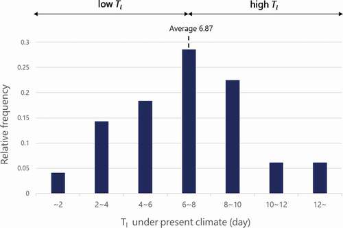
Figure 13. Scatter diagrams of the time period from genesis to landfall (Tl) derived from JMA best track and the central pressure (Pc) for target typhoons calculated from: (a) present-climate experiments and (b) future-climate experiments. (c) A scatter diagram of Tl and future changes in Pc between (b) future and (a) present climates. In (a) and (b), the Orange and purple points represent cases where rapid intensification (RI) did and did not occur, respectively. In (c), the Orange and purple points represent cases where RI occurs under only the future climate and all other cases, respectively. Green lines in the diagrams represent regression lines.
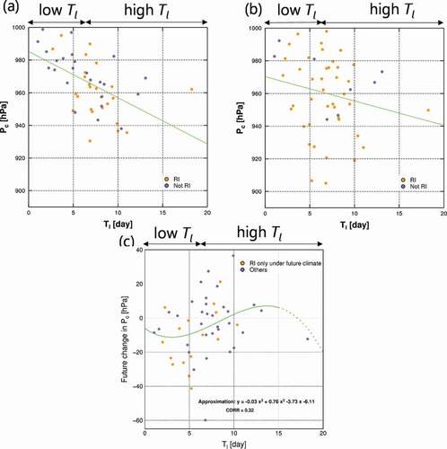
Figure 14. Relative frequency distribution of the radius of maximum wind speed at landfall times (Rml) for target typhoons in the present-climate experiments. The average values of Rml for all cases is 101.4 km. Cases with values of less than 101.4 km are referred to as small Rml, whereas cases with values equal to or larger than 101.4 km as large Rml.
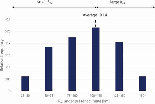
Table 5. Central pressure values (Pc) averaged for all (49 cases), small Rml (23 cases), and large Rml (26 cases) in PGWDs. Typhoons with Rml of less than 101.4 km are referred to as “small Rml” (23 cases), whereas those with Rml of 101.4 km or more as “large Rml” (26 cases). The left, middle, and right columns show the average values for the present-climate experiments, future-climate experiments, and future changes, respectively. The values in parentheses indicate the standard deviation
Figure 15. Scatter diagrams of the radius of maximum wind speed (Rml) under present climate and central pressure (Pc) for target typhoons calculated from: (a) present-climate experiments and (b) future-climate experiments. (c) A scatter diagram of Rml and the future changes in Pc. The points correspond to those provided in .
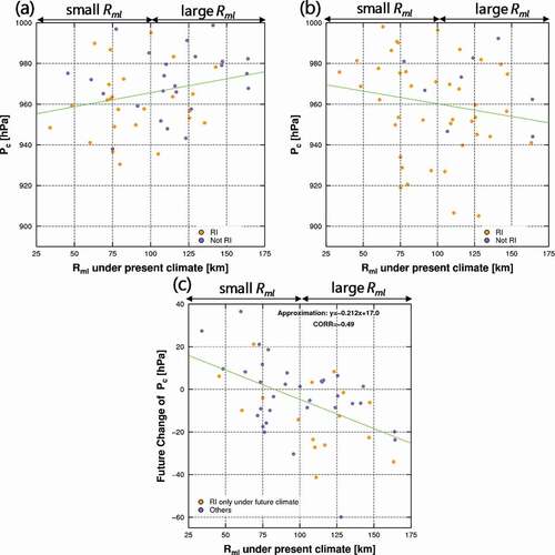
Figure 16. Computational flow of the e-PGWD method. The left, middle, and right columns show the flows of the present-climate experiment, future-climate experiment (e-PGWD), and horizontal resolution at each calculation step, respectively.
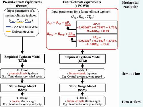
Figure 17. Scatter diagram of future-climate central pressure (Pc) in PGWDs (horizontal axis) and e-PGWDs (vertical axis).
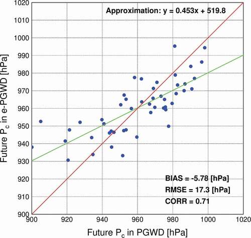
Figure 18. (a) The scatter plot between Tl and future change of Rml (ΔRml.). The scatter plot between Rml under present climate and future change of Rml (ΔRml). The correlation coefficient is 0.24 for Tl and ΔRml and −0.61 for Rml under the present climate and ΔRml.
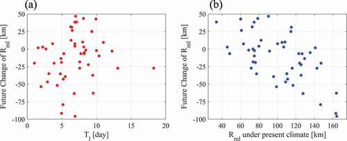
Figure 19. Horizontal distributions of the ocean topography around (a) Ise Bay and Mikawa Bay, and around (b) Osaka Bay are used in the storm surge model (SSM). The red points indicate the target ports for validating and discussing the SSM results: (a) Port of Nagoya and (b) Port of Osaka.
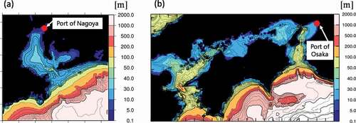
Table 6. Attribute variables for three target typhoons in 2018 (Typhoons Jongdari, Jebi, and Trami) used for e-PGWD: input typhoon parameters (Pc,Tl, and Rml), estimated future typhoon changes (∆Pc and ∆Rml), and estimated future typhoon parameters (Pcf and Rmlf) with standard errors of estimation (Pce and Rmle)
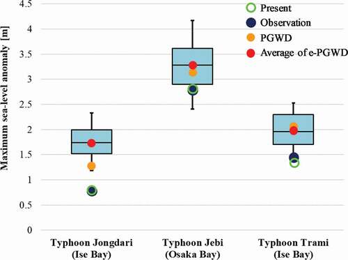
Figure 20. Box-and-whisker plot of the maximum sea-level anomalies at the target port simulated by e-PGWDs for nine cases. The blue, dark-blue, Orange, and red points indicate the maximum sea-level anomalies at the target port simulated by the observations (black points), present-climate experiments (green points), PGWD results by HTM (Orange points), and average values for all e-PGWDs. The box height includes the half of all the ensemble sizes in e-PGWDs, and the black line in the box represents the median value.