
Figures & data
Table 1. Experimental parameters applied to acquire T1- and T2-weighted images of paramagnetic nanoformulations using an MRI scanner.
Figure 1. Characterization of Ferritis, Gadolinis and Manganis nanoparticles. (A) TEM images of each type of nanoparticles. (B) DLS characterization of Z-average, PDI (polydispersity index) and zeta potential. All measurements were performed in triplicates, and data are presented as mean ± SD. (C) EDS images displaying metal distribution (Fe, Gd or Mn) throughout the nanoparticles.
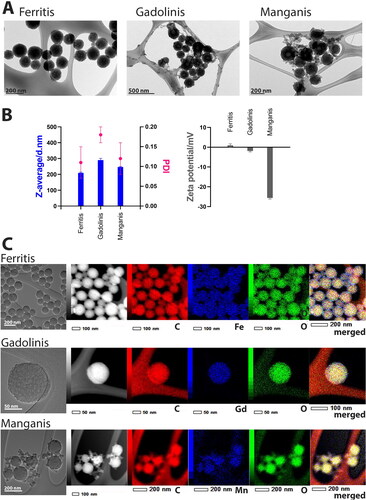
Figure 2. SQUID measurements of MPDA NPs, Ferritis, Gadolinis and Manganis NPs. (A) Magnetic susceptibility. (B) Magnetization at 2 K. (C) Magnetization at 300 K.
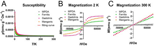
Figure 3. Relaxivity (R1) evaluation of (A) Ferritis, (B) Gadolinis and (C) Manganis nanoparticles at 22 and 37 °C measured using a 16.5 MHz (0.4 T) spectrometer.
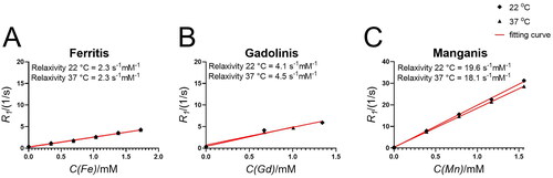
Figure 4. T1 contrasting properties of (A, B) Ferritis, (C, D) Gadolinis and (E, F) Manganis nanoparticles measured using a 9.4 T MRI spectrometer. The left images are T1-weighted images obtained using the MRI scanner at different τ values, whereas the right graphs are the corresponding T1 times extracted from the maps.
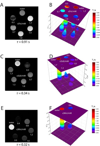
Figure 5. T2 contrasting properties of (A, B) Ferritis, (C, D) Gadolinis and (E, F) Manganis nanoparticles measured using a 9.4 T MRI spectrometer. The left images are T2-weighted images obtained using the MRI scanner, whereas the right graphs are the corresponding T2 times extracted from the maps.
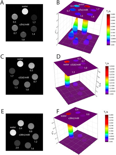
Figure 6. Photothermal evaluation of (A) Ferritis, (B) Gadolinis and (C) Manganis nanoparticles solutions in water measured using a thermocouple.
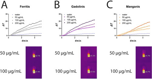
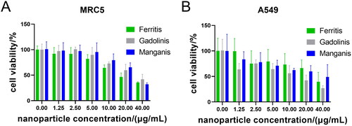
Figure 7. Cytotoxicity study. WST-1 assay results of Ferritis, Gadolinis and Manganis NPs incubated with (A) normal cells (MRC-5) and (B) cancer cells (A549).
Supplemental Material
Download MS Word (379.6 KB)Data availability statement
All data generated or analysed during this study are included in this published article (and its Supplementary Information files).