Figures & data
Figure 1. Durrães railway bridge: a) overview; b) railway track.
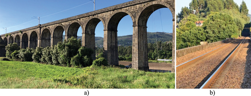
Figure 2. Durrães railway bridge: details of the longitudinal cracks on the intrados of arch A15.
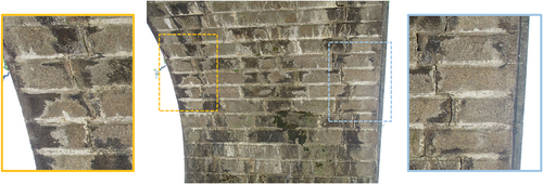
Figure 3. Experimental setups of the ambient vibration tests: a) global test; b) local test.
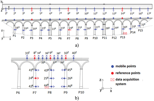
Table 1. Technical specifications of the accelerometers.
Figure 4. Ambient vibration test: average normalized singular values of the spectral density matrices of all test setups.
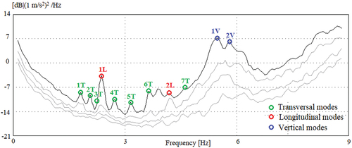
Table 2. Experimental frequencies and damping coefficients identified for Durrães bridge.
Figure 5. Experimental modal configurations.
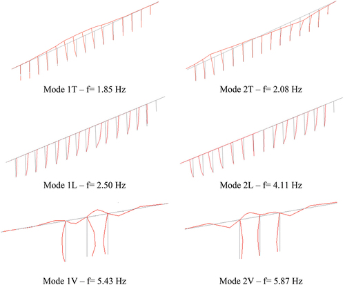
Figure 6. Static load tests: experimental setup.
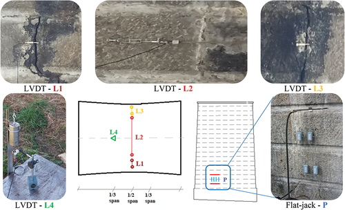
Figure 7. Static load tests: a) position 1.1; b) position 1.2; c) position 2.1; d) position 2.2.
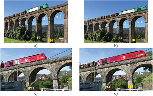
Figure 8. Dynamic test: a) setup measurement points in arches and piers (distances in meters); b) accelerometer on the deck; c) accelerometer on the pier.
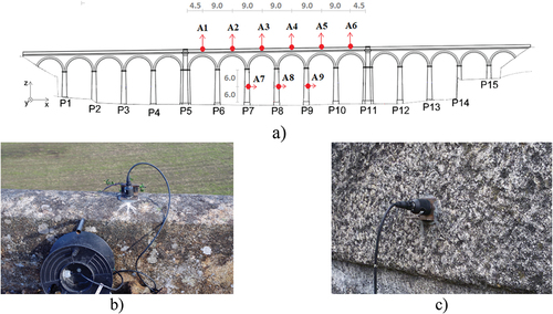
Figure 9. 3D global numerical model of Durrães bridge [Citation39].
![Figure 9. 3D global numerical model of Durrães bridge [Citation39].](/cms/asset/0b2b0baf-1833-4ab9-9427-861423fb4106/tjrt_a_2133783_f0009_oc.jpg)
Table 3. Elastic and mass parameters of the FE model of Durrães bridge.
Figure 10. Comparison between some of the numerical and experimental global modal parameters of Durrães bridge.
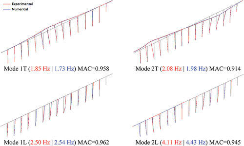
Figure 11. 3D local numerical model of Durrães bridge: a) arch A15 and adopted contact model; b) location of contact/target elements on both spandrel walls interfaces; c) location of contact/target elements on other interfaces.
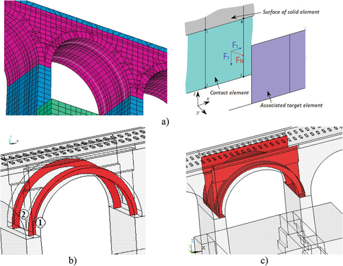
Figure 12. Contact model behaviour: a) normal direction; b) tangential direction.
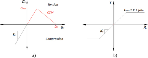
Table 4. Contact elements’ parameters.
Figure 13. Material model behaviour: a) exponential hardening and softening in compression; b) exponential softening in tension.
Table 5. Drucker-Prager (D-P) model parameters.
Figure 14. Comparison between the numerical and experimental local vertical modal parameters of Durrães bridge.
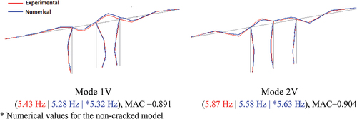
Figure 15. Takargo freight train: a) general view; b) loading scheme (dimensions in metres and static loads in kN); c) train dynamic signature.
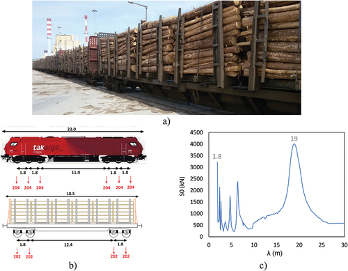
Figure 16. Freight train FE model: a) Sgnss waggon, b) bogie detail.
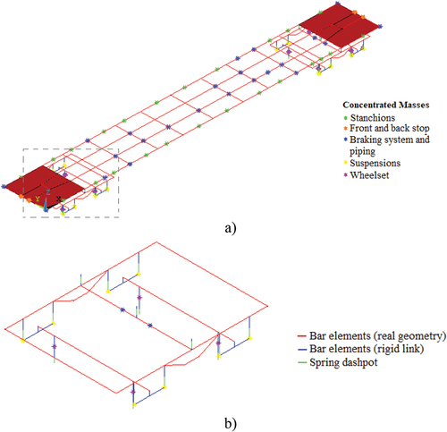
Table 6. Main parameters of the numerical model of Sgnss vehicle (loaded configuration).
Figure 17. Comparison between some of the numerical and experimental modal parameters of Sgnss wagon (loaded configuration).
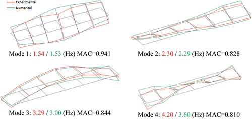
Figure 18. Train–bridge interaction model: a) overview; b) detail of the wheel-rail contact and c) contact/target pair scheme.
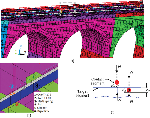
Table 7. Key options set for the contact-pair model [Citation51].
Figure 19. Irregularities profile on Durrães bridge: a) longitudinal levelling b) auto-spectra amplitude.
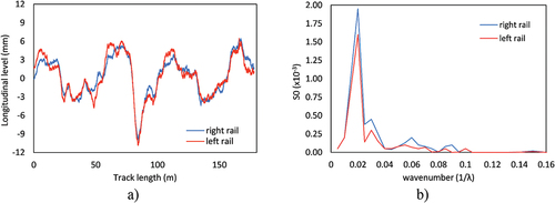
Figure 20. Loading cases for the static numerical analysis.
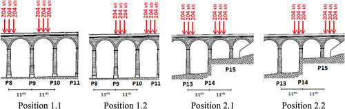
Figure 21. Experimental vs Numerical static vertical displacements: a) load test 1 (positions 1.1 and 1.2); b) load test 2 (positions 2.1 and 2.2).
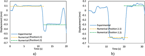
Figure 22. Stress variation on the bridge piers under permanent and live loads for pier P11 and P14: a) and b) experimental results; c) and d) numerical results.
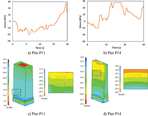
Figure 23. Experimental and numerical crack opening values on the spandrel wall interfaces of arch A15: a) on the side of transducer L1; b) on the side of transducer L3.
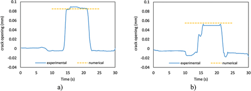
Figure 24. Dynamic responses for the passage of the freight train at 60 km/h at mid-span of the arches in the vertical direction: a) accelerations time series, b) PSD amplitude, c) train dynamic signature.
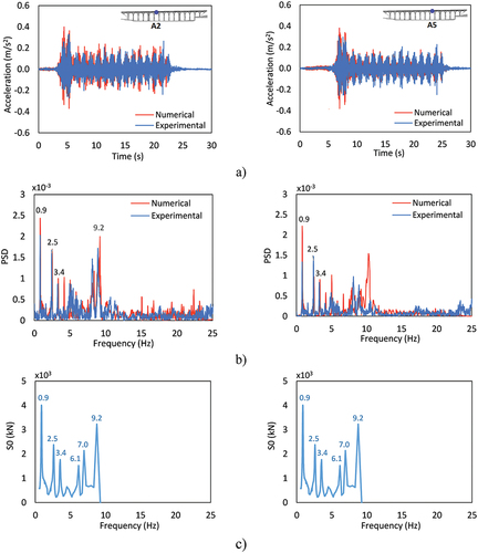
Figure 25. Dynamic responses for the passage of the freight train at 60 km/h at half-height of piers in the longitudinal direction: a) acceleration time series, b) PSD amplitude, c) train dynamic signature.
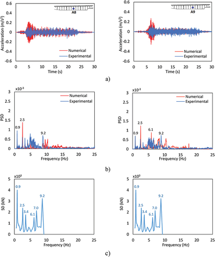
Figure 26. Plastic strain level in terms of principal maximum strains (in ‰) for the freight train passage at 60km/h: a) arch A9; b) arch A15.
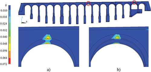
Figure 27. Maximum vertical dynamic response of several arches of Durrães bridge for the passage of the freight train for speeds between 40 km/h and 140 km/h in terms of: a) displacements; b) accelerations.
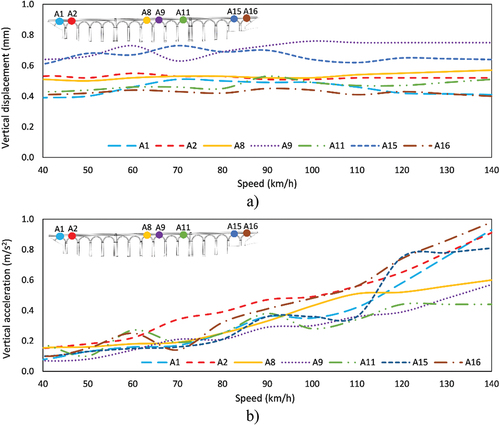
Figure 28. Crack opening values on the spandrel wall interface of arch A15 due to the freight train passages at 60, 80, 100, 120 and 140 km/h.
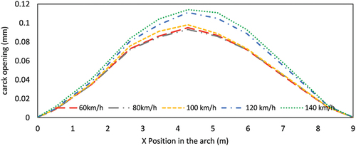
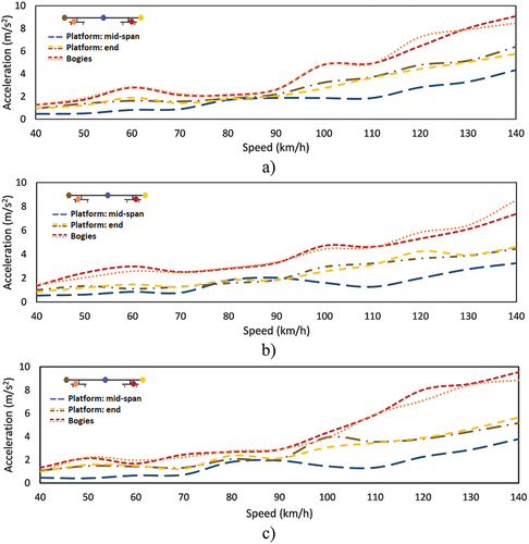
Figure 29. Maximum vertical accelerations at different points of the waggon’s platform for the: a) first waggon, b) intermediate waggon, c) last waggon.