Multi-scenario Extreme Weather Simulator application to heat waves: Ko’olauloa community resilience hub

Figures & data

Fig. 1. Overview of MEWS and BEM study process. Ovals portray analysis inputs and boxes indicate steps. The left-hand-side process is only executed once for historical fits, while the right-hand-side process is executed over SSP scenario, future year, HW FDI confidence interval, BEM model, and realization number.

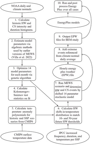
Table 1. IPCC HW intensity and frequency multiplying factors from Masson-Delmotte et al. (2021, Figure SPM.6).

Event	$\mathrm{\Delta }{T}_S$ (⁰C)	5% ΔT (⁰C)	50% ΔT (⁰C)	95% ΔT (⁰C)	5% $\Delta f$	50% $\Delta f$	95% $\Delta f$
HW 10-year event	1.0	0.7	1.2	1.5	1.8	2.8	3.2
	1.5	1.3	1.9	2.3	2.8	4.1	4.7
	2.0	1.8	2.6	3.1	3.8	5.6	6
	4.0	4.3	5.1	5.8	8.3	9.4	9.6
HW 50-year event	1.0	0.7	1.2	1.6	2.3	4.8	6.4
	1.5	1.3	2	2.4	4.3	8.6	10.7
	2.0	1.8	2.7	3.2	6.9	13.9	16.6
	4.0	4.4	5.3	6.0	27	39.2	41.4

Surface temperature change is the shift from 1850 to 1900 mean.

Fig. 2. Time-dependent probability function for HW and CS events.

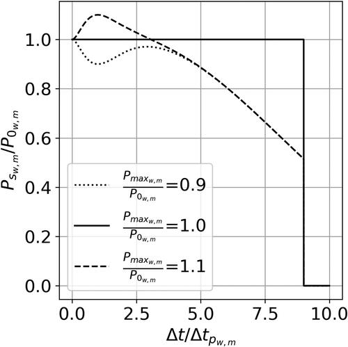
Fig. 3. Major locations and geology of Oahu, Hawaii, adapted from Dores and Lautze with permission (Dores and Lautze 2020).

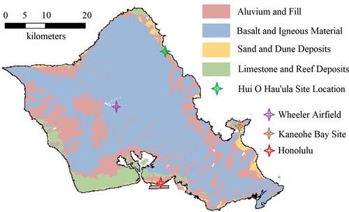
Table 2. KCRH design cases used to quantify energy efficiency.

Design aspect	BAU	HE
A/C	Direct expansion (DX) coils for single-duct air terminals with dampers and reheat.	Centralized chilled water coils. Same duct configuration as BAU. High-efficiency variable-speed fans, an outdoor air economizer, and heat exchange between exhaust air and incoming outdoor air. The control includes a supply air temperature reset ranging from 10 to 12ºC based on the warmest thermal zone temperature.
Cooling source	DX packaged rooftop unit for heating and cooling with humidity control. No special considerations in efficiently servicing critical loads.	Connected systems: two water source chillers with a ground heat exchanger (GHE) and air-to-water heat rejection. Redundancy for critical loads is provided with either chiller being able to serve them. Also the GHE can reject heat of critical loads without air-to-water heat rejection.
Refrigeration	16 m^2 walk in refrigerator with air-source heat rejection	Connected system: 16-m^2 walk-in refrigeration with water-source heat rejection connected to chiller cooling water (CW) loop
Ventilation	1 common ventilation system, mechanical ventilation in gym	Two ventilation systems fully separating critical and noncritical loads, natural ventilation in gym
Lighting	5 W/m^2 (normal LED performance)	3 W/m^2 (high light-emitting diode [LED] performance with well-coordinated daylighting)
Fans	61% efficiency	80% efficiency
Pumps	90% efficiency	95% efficiency
Walls	1.35 m^2K/W average R value	2.79 m^2-K/W average R value—also interior walls surrounding critical load spaces given exterior insulation for all surfaces
Roof	ASHRAE 189 climate zone 1 exterior roof with 3.9 m^2K/W	Cool roof (solar absorptance of 0.45) with 6.97 m^2-K/W resistivity
Windows	Average U-factor of 4 W/m^2/K, solar heat gain coefficient (SHGC) 0.3, visible light transmittance (VLT) 0.3	Average U-factor of 1 W/m^2-K, SHGC of 0.23, and VLT of 0.4
Doors	25-mm insulation board	R18 (3.2 m^2K/W) + 25 mm insulation board
Waste heat exchange	None	Outside air to exhaust air heat exchanger and sewage water heat recovery
Hot water	Electric element	Heat pump water heater (HPWH) with backup electric element and thick insulation. The HPWH cools mechanical space and indirectly draws waste heat from other equipment.

To obtain both of these models, go to https://github.com/sandialabs/MEWS. Then navigate to “examples,” then to “example data,” then to “HuiOHauula.” The BAU case is in “ep_models” and the HE case is in “ep_models.”

Table 3. Differences between NormOps and ResOps.

Design aspect	NormOps	ResOps
A/C	All spaces cooled except gym, side stairs, mechanical room, and freight elevator	Only cool the following critical spaces: Level 1: kitchen, food storage; Level 2: medical, security; Level 3: staff area, conference room.
Hot water	Available	None
Refrigeration	Walk-in, two stand-alone refrigerators and two stand-alone freezers	Only walk-in
Occupancy	Peak occupancy of 70 people each day with a daily average of 38 people	Four times the occupancy with peak of 282 people and daily average of 153. Gym and critical spaces are occupied at night
Plug loads	11.38 W/m2	Same amount. This implies rationing of plug loads to a larger group of people but with no increase.
Medical	Medical center without dialysis	Medical center + 3 Tablo hemodialysis systems (Tablo 2023) being used during the day (intensive but not 24/7)

Table 4. Changes added to Kane’ohe Bay TMYx 2004–2018 EPW file.

Variable	Change description
Dry-bulb temperature	Optimized offset and multiplicative parameters to match monthly climate average maximum and minimum values from Weather Spark’s webpage for Hau’ula to hourly Kane’ohe Bay TMYx (WeatherSpark 2023).
Dew-point temperature	Changed values to be consistent with updated dry-bulb temperature and unchanged relative humidity.
Radiation (direct and diffuse)	Adjusted Kane’ohe Bay TMYx 2004–2018 hourly values so that monthly average, hour-of-day global horizontal radiation values from University of Hawaii (Giambelluca et al. 2014) match for the latitude and longitude of the site.
Ground temperatures	Shifted ground temperatures down by 3.03 °C to make the average of 3-, 4-, and 5-m-deep readings in the TMYx file match ground water temperature of 21.7 °C reported by Dores and Lautze (2020) for Hau’ula

Table 5. NOAA data characteristics.

Input	Value
Station location	Kane’ohe Bay
Station ID	USW00022519
Climate norms	1991–2020
Daily summaries	1942–2023
Filtering	Daily summaries required gap filling using a SARIMA model

Fig. 4. KCRH in Hau’ula, HI, EnergyPlus model with three levels: (A) isometric view showing covered parking, (B) lower floor, (C) main entrance floor, and (D) upper floor. The design is by + Lab Architect PLLC (Azaroff 2023).

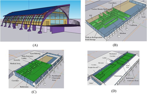
Fig. 5. Shared heat rejection.

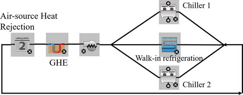
Fig. 6. Gap-filled NOAA daily summaries.

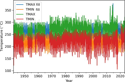
Table 6. Kolmogorov–Smirnov test statistics for MEWS Kane’ohe Bay fit.

	Duration				Temperature
Month	HW		CS		HW		CS
	Statistic	p Value	Statistic	p Value	Statistic	p Value	Statistic	p Value
1	0.023092	0.999775	0.115327	0.001477	0.200695	7.456524e-08	0.157785	0.000003
2	0.078382	0.230246	0.114468	0.004146	0.137200	2.811642e-03	0.124873	0.001286
3	0.070624	0.379734	0.094384	0.008577	0.170377	1.474030e-04	0.076134	0.057162
4	0.086225	0.192003	0.070097	0.069220	0.138662	4.877060e-03	0.114668	0.000255
5	0.068583	0.403028	0.092746	0.006257	0.112478	2.867868e-02	0.059037	0.190783
6	0.093537	0.159609	0.070157	0.078387	0.250759	2.765237e-08	0.139464	0.000006
7	0.131092	0.002089	0.059334	0.181783	0.196401	4.047055e-07	0.096573	0.003609
8	0.111761	0.011250	0.127836	0.000047	0.199154	1.443825e-07	0.123753	0.000091
9	0.120070	0.062826	0.084999	0.009526	0.173652	1.478366e-03	0.136081	0.000002
10	0.078358	0.172331	0.089130	0.005178	0.138592	9.849804e-04	0.123505	0.000022
11	0.103622	0.021321	0.045475	0.481458	0.100676	2.746377e-02	0.105592	0.001085
12	0.087386	0.072944	0.090776	0.023918	0.142417	3.144755e-04	0.074269	0.102565

Ninety-five percent confidence is equivalent to the p value being greater than 0.05. Values failing the test are shown in red. The “Statistic” columns give the maximum difference in cumulative distribution functions of the historic distribution versus the MEWS fit.

Fig. 7. June MEWS fits to temperature (a) and duration (c) and shift and stretch for SSP 5–8.5 for 2080 and 95% HW CI (b).

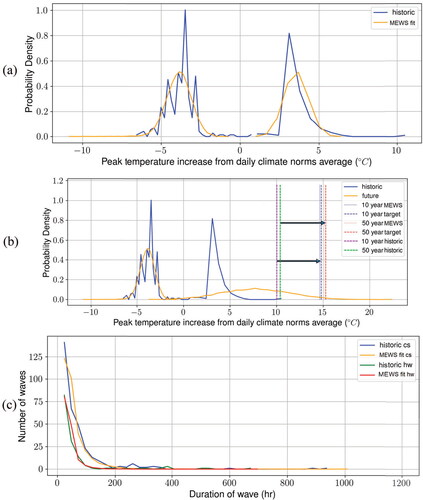
Fig. 8. CMIP6 polynomial fits to surface temperature at the KCRH site.

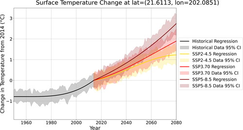
Table 7. CMIP6 polynomial coefficients $t\mathrm{ }$= year − 2014.

	$t^6$	$t^5$	$t^4$	$t^3$	$t^2$	$t$	$1$
Historical	−1.8231e-12	−7.0498e-10	−7.2341e-08	2.6166e-06	8.2021e-04	4.4934e-02	−4.7280e-06
SSP2-4.5	0	0	0	−5.9508e-06	5.2949e-04	9.5840e-03	−2.2866e-07
SSP3-7.0	0	0	0	−2.3118e-06	3.5316e-04	1.5495e-02	−2.2594e-07
SSP5-8.5	0	0	0	7.1558e-07	1.6873e-04	2.7302e-02	−7.8113e-08

Fig. 9. Statistical moments of dry-bulb temperature (°C) for 7,200 weather files. The x axis is °C or $\mathrm{\Delta }$°C for all plots.

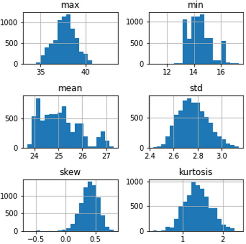
Table 8. EUI results for all four models.

EUI (1915 m^2), kWh/m^2/yr	Business-as-usual configuration (BAU)	High-efficiency configuration (HE)	Energy savings (%)
NormOps	189.95	118.92	37.39
ResOps	122.20	90.32	26.07

Table 9. Hawai’i Energy Utility Benchmarking (HEUB) data (HEUB 2023).

EUI, kWh/m^2/yr	Minimum	Average	Maximum	Number of samples
Grocery stores	129	530	690	33
Office buildings	86	170	290	60
Restaurants	48	350	650	14
Hotels	21	110	200	27

Fig. 10. Average percent hours within four temperature ranges. C = caution, 32.2 °C < T ≤ 26.7 °C; D = danger, 32.2 °C < T ≤ 39.4 °C; EC = extreme caution, 39.2 °C < T ≤ 51.7 °C; ED = EXTREME Danger, T > 51.7 °C. Rows vary by SSP and columns by operation type.

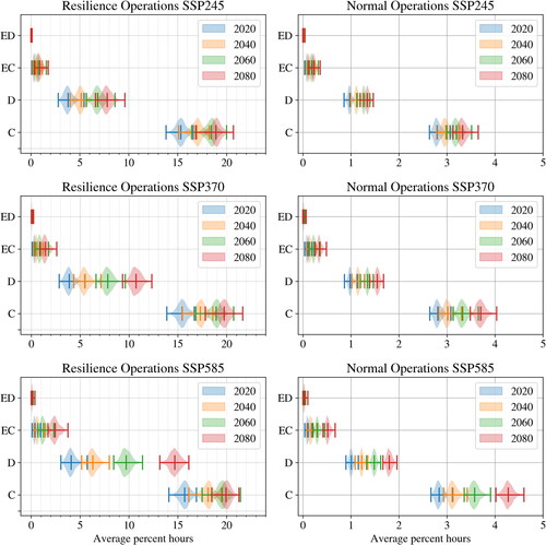
Fig. 11. EUI by operation mode, year, and SSP (colors according to legend in Figure 9). The y axis is probability density.

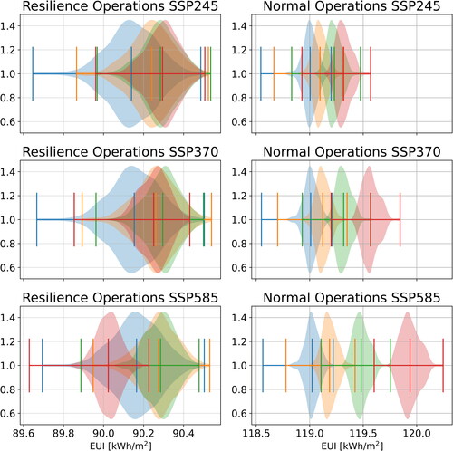
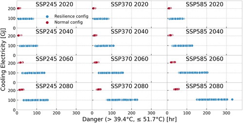
Fig. 12. Cooling energy vs. average dangerous hours by operation mode, year, and SSP.

Masson-Delmotte, V., P. Zhai, A. Pirani, S. L. Connors, C. Péan, S. Berger, N. Caud, Y. Chen, L. Goldfarb, M. I. Gomis, et al., eds. 2021. Technical summary. In Climate change 2021: The Physical science basis. Contribution of working group I to the sixth assessment report of the Intergovernmental Panel on Climate Change, 135–144. Cambridge, UK: Cambridge University Press. doi: 10.1017/9781009157896.002.

 Google Scholar

Dores, D., and N. Lautze. 2020. Preliminary assessment of ground-source heat exchangers for cooling in Hawai‘i. Sustainable Energy Technologies and Assessments 37:100579. doi: 10.1016/j.seta.2019.100579.

 Web of Science ®Google Scholar

Tablo. 2023. Tablo hemodialysis unit web page. Accessed June 6, 2023. https://www.outsetmedical.com/tablo.

 Google Scholar

WeatherSpark. 2023. Climate and average weather year round in Hau’ula Hawaii. Accessed September 5, 2023. https://weatherspark.com/y/137/Average-Weather-in-Hau%E2%80%98ula-Hawaii-United-States-Year-Round.

 Google Scholar

Giambelluca, T. W., X. Shuai, M. L. Barnes, R. J. Alliss, R. J. Longman, T. Miura, Q. Chen, A. G. Frazier, R. G. Mudd, L. Cuo, et al. 2014, February. Evapotranspiration of Hawai‘i. Final report submitted to the U.S. Army Corps of Engineers—Honolulu District, and the Commission on Water Resource Management, State of Hawai‘i. Technical Report. http://evapotranspiration.geography.hawaii.edu/assets/files/PDF/ET%20Project%20Final%20Report.pdf.

 Google Scholar

Azaroff, I. 2023. +Lab Architect PLLC website. https://www.pluslabglobal.com/.

 Google Scholar

HEUB. 2023. Hawai’i Energy Utility Benchmarking data website. https://hawaiienergy.com/for-business/benchmarking-by-facility-type.

 Google Scholar