Newly uncovered physics of MHD instabilities using 2-D electron cyclotron emission imaging system in toroidal plasmas

Figures & data

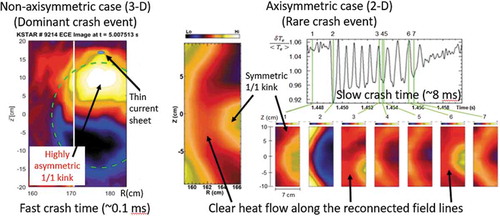
Figure 1. Schematics of magnetically confined plasma in (a) tokamak and (b) stellarator configuration. In tokamak configuration, the rotational transform (helically twisted magnetic field) is formed by both the toroidal field by external coils and poloidal field induced by the toroidal plasma current. In stellarator configuration, the rotational transform is produced entirely by non-axisymmetric external coils.

Source: Y. Xu, Matter and Radiation at Extremes, 1, 192e200, 2016, [email protected].

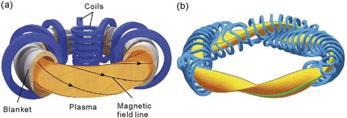
Figure 2. Illustration of double inversion process of the measured Faraday rotation angles using 9 chords of probe beams. In order to increase the precision, radial jogging of the plasma was performed as shown in the plot of line densities and Faraday rotation angles (left side). Then Abel inversion is introduced to invert the line integral density into the local density. Then the local density profile is used to evaluate the poloidal field which is used to calculate safety factor profile (right side).

Source: partial figure from H. Soltwisch

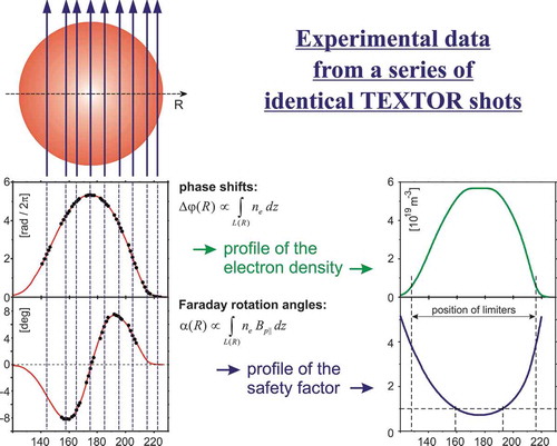
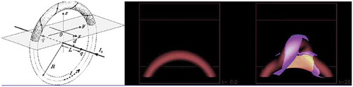
Figure 3. A schematic of MSE viewing geometry for edge and center of the plasmas on DIII-D tokamak (left side). Viewing angles with respect to the plasma are shown with typical positions of the axis and separatrix are ~1.55m and ~2.13m, respectively. The MSE measured poloidal field (B_z) and B_z from equilibrium reconstruction (solid line) are compared just before the sawtooth crash. The q profiles for before (q₀ = 0.97) and after (q₀ = 1.05) the sawtooth crash are ploted.

Source: B.W., Rice, Fusion Engineering and Design, 34–35, 1997

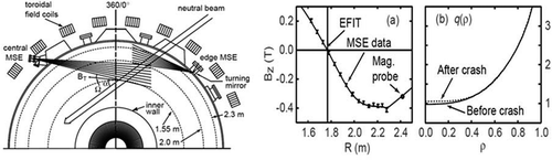
Figure 4. (a) Arrangement of the conventional 1-D ECE system for T_e profile measurement is illustrated. The system utilizes a single detector and wideband sweeping local oscillator source for single row of sampling volumes with a typical resolution of ~5 cm x ~ 5 cm. (b) Arrangement of the 2-D ECEi system with a quasi-optical 1-D vertical detector array with large optics (triplet lens system). Each detection element consists of Schottky diode and dipole antenna is like a single mixer in the 1-D ECE system and 2-D array of sampling volumes is formed within the focal depth of the optical system. The down converted IF signal is splitted into 8 radial channels to form radial profile of T_e at a given vertical position.

Source: Park, H,

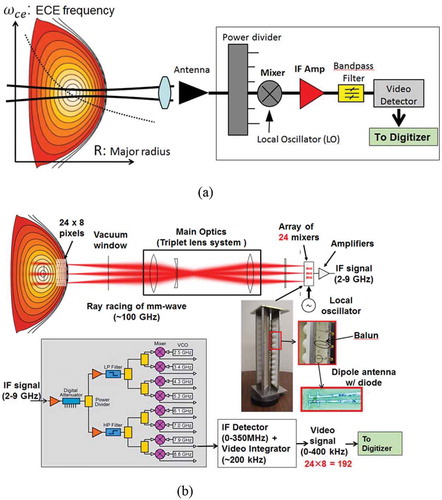
Figure 5. Demonstration of the sawtooth crash event by the first 2-D ECEi system on TEXTOR tokamak plasma. A time trace of the central channel of the ECEi system shows sawtooth oscillation in different time scales (slow rise and fast crash). The captured 2-D images of δT/<T_e> before (1), during (2) and after (3) the sawtooth crash, are illustrated with the q ~ 1 layer (white double line). Before the crash, symmetric and peaked T_e profile is shown in the frame 1. During the crash phase, a hint of heat flow is shown in the mixing zone in the frame 2. Heat from the core is accumulated in the mixing zone and T_e is flattened within q ~ 1 surface (double white line).

Source: H. Park

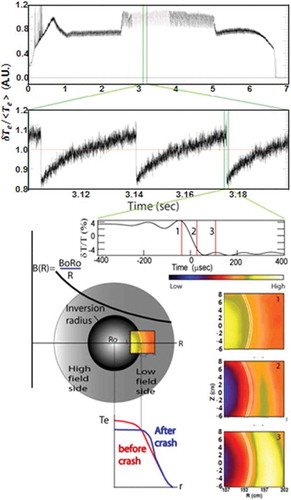
Figure 6. Arrangement of the KSTAR quasi 3-D ECEi system is illustrated. The 1st ECEi system equipped with two views for simultaneous measurement at two poloidal planes (e.g. core/edge or high field side/low field side) is shown in red color box. The 2nd ECEi system with blue color is added at the toroidal plane separated by 22.9° and simultaneously measured ELM images from two edge views are shown. Here, the pitch angle, velocity and mode numbers can easily be calculated.

Source: H. Park

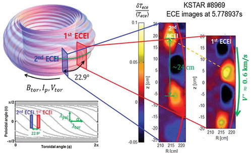
Figure 7. The measured electron temperature and q₀ by MSE system on KSTAR are shown. The measured average value is ~1.0 and variation of the q₀ (δq) before and after the crash is ~0.06 with error range of $\pm 0.03$.

Source: Y. B. Nam, et al Nucl. Fusion 58, 066009, 2018, Figure 1

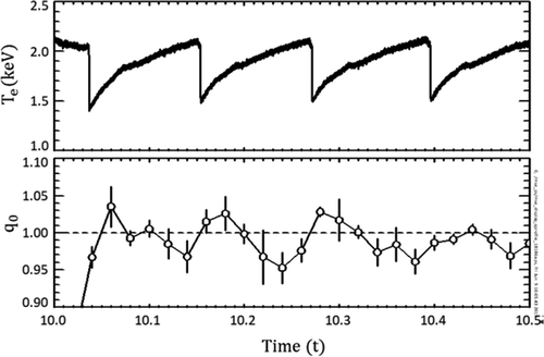
Figure 8. Illustration of 2-D images of the fast crash process at the high (a) and low (b) field side of q ~ 1 surface (black line) of the TEXTOR plasma where the center of the plasma is ~177 cm. The time trace is from (z = 0) near the q ~ 1 surface from both sides. Ballooning type of bulge with a clear ‘finger’ is shown at both sides. Severe distortion (or harmonic generation) of the 1/1 kink mode prior the crash at both sides is shown.

Source: partial figure from H.K. Park, et al Phys. Rev. Lett. 96 195,003, 2006 (a)

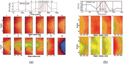
Figure 9. Comparison of the reconstructed images with 1-D ECE when the hot spot is on the good curvature side and on the bad curvature side. (a) The contour plot of the electron temperature profile; the contour step size is 250 eV, and the hatched region indicates T_e ~56–6.25 keV. (b) The contour plot of the temperature difference; the contour step size is 100 eV and the hatched region indicates less than 300 eV. (c) The contour plot of the perturbation of the electron temperature; the contour step size is 60 eV. The dashed circles indicate, 1- the mixing radius, 2- the inversion radius. The regions indicate, 3-the hot spot, 4- the island, and, 5- the cool region between the hot spot and the island.

Source: Y. Nagayama, Physics of Plasmas 5, 1647 (1996) Figure 5

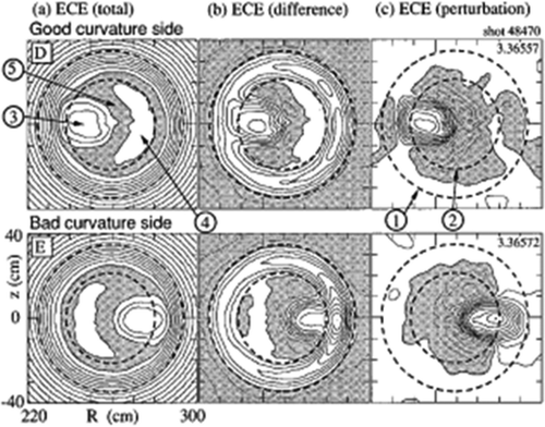
Figure 10. The measured 2-D images of the hot spot (1/1 kink mode) and cold region (island) are directly overlaid for comparison with the 2-D contour patterns from (a) the full reconnection model and (b) the quasi-interchange model.

Source: H.K. Park, et al Phys. Rev. Lett. 96, 195,004, 2006

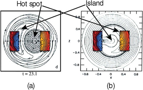
Figure 11. The 2-D images during the sawtooth crash event from (a) EAST, (b) ASDEX-U and (c) HT-7 are similar to those from the TEXTOR. The rotating 1/1 kink mode is observed prior the crash time and the core heat inside the 1/1 kink mode is transported through the localized reconnection zone and the transported heat is piling up in the mixing zone after the crash. Highly distorted 1/1 kink modes are commonly illustrated in the images of the sawtooth crash in all devices. The level of distortion of the 1/1 kink mode can be represented as a harmonic generation.

Sources:a.EAST: Gao, B.X., et al JINST 13, P02009, 2018b.ASDEX-U: Igochine, V., et al Phys. of Plasma, 17, 122,506, 2010c.HT-7: Wan, B., et al Nucl. Fusion, 49, 10, 2009 Figure 21

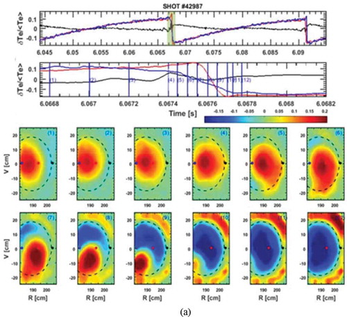
Figure 11. (Continued).

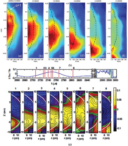
Figure 12. (a) The modelled q profiles inside the q ~ 1 surface with a dip in the q profile at r/a = 0.2 for three different q₀ values (0.8, 0.98 and 1.04) are shown in the left side. Maximum growth rates of the resonant modes calculated using M3D-C¹ code are shown in the right side as the dip in the q profile with q₀ = 1.04 is scanned from the center to the edge of the q ~ 1 surface (zone 1, 2, 3, and 4). (b) Excited resonant mode is shown when the current blip (dip in the q profile) is scanned from the center of the plasma to the edge of the q ~ 1 using ECCD. In zone 1 (r/a < 0.15), a hot spot in the core is observed. In zone 2 (0.1< r/a < 0.22), the 2/2 mode is excited. In zone 3 (0.2< r/a < 0.27), the 3/3 mode is observed. Near the q = 1 region, higher order mode is excited.

Source: Nam, Y.B., et al Nucl. Fusion 58, 066009, 2018, Figure 2, Figure 3

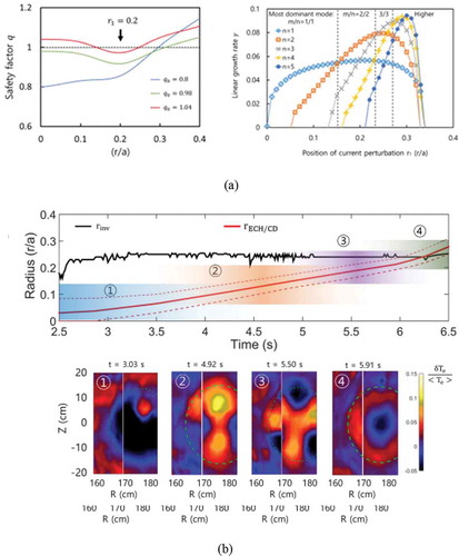
Figure 13. One sawtooth period without and with the current blip is compared. The sawtooth without current blip only has the 1/1 kink mode just before crash (upper left). One sawtooth cycle with the current blip in zone 3 in Figure 12, has the 3/3 mode in early rising phase after the crash. The 3/3 mode transforms into the 2/2 and 1/1 mode before the crash. The 2-D images of the 3/3, 2/2 and 1/1 mode are shown in the right side. The transformation is likely due to the change of the background q value as the current builds up with the increasing T_e in the core.

Source: Nam, Y.B., et al Nucl. Fusion 58, 066009, 2018, Figure 4

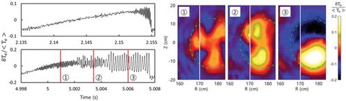
Figure 14. (a) The 2-D images of the ‘post-cursor’ case at high field side are shown with the time trace of T_e to demonstrate that the reconnection time scale is an order of magnitude longer compared to the fast reconnection events (TEXTOR data). Prior to the crash, the 1/1 kink mode is nearly symmetric (frame 1) and partial heat is transported to the mixing zone after the first crash (frame 2). The reconnected field lines of the remnant 1/1 kink mode are clearly illustrated in the frames 3 and 4. (b) The contour plot of T_e illustrates that the 1/1 kink mode is connected to the q ~ 1 surface with the reconnected field lines. (c) The measured reconnected field lines of the 1/1 kink mode at the high field side and cold island at the low field side are overlaid on the reconstructed crash model.

Source: Park, H.

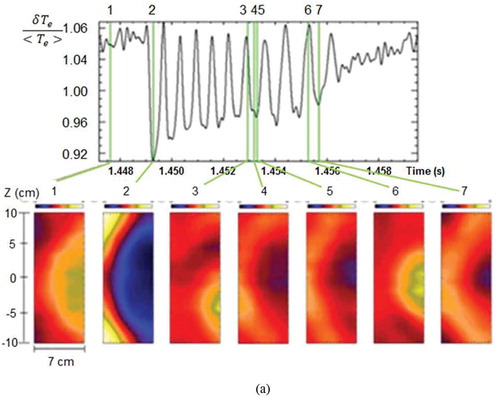
Figure 14. (Continued).

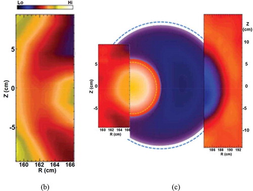
Figure 15. (a) The crash event with a fast reconnection time is dominant in sawtooth crashes. They exhibit highly distorted 1/1 kink mode (higher harmonics in poloidal and toroidal planes) and initial reconnection is likely on the tip of the ‘finger’ as shown in the image from KSTAR (examples in Figures 8 and 11a-11c) (i.e., 3-D nature). (b) The crash time of the ”post-cursor” case shown in Figs. 14 and 15b, is an order of magnitude slower compared to that of the fast crash cases. The reconnection zone is much wider on poloidal plane and it is toroidally axisymmetic (i.e., 2-D nature). Slow reconnection time case resembles the Sweet Parker model and fast reconnection time case fits to the Petschek model.

Source: Park, H.

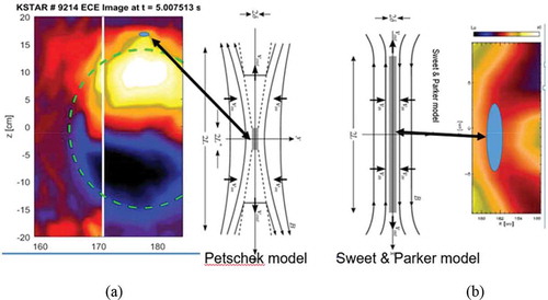
Figure 16. Schematic of the position and shape of the example NTMs (2/1, 3/1 and 4/1) on KSTAR geometry. Two figures of NTMs represent O-point (left) and X-point (right) on the mid-plane, repectively.

Source: G, Kim

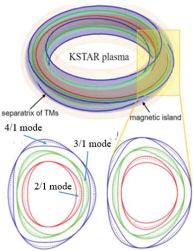
Figure 17. (a) The 2-D image consist of 192 pixels (24 x 8) in the vicinity of the 2/1 mode is shown with the equilibrium constructed by EFIT on (R, Z) coordinate of KSTAR. (b) Four images of the 2/1 mode at different phase are plotted as it rotates (see the 2/1 mode in Figure 16) with the X-point and O-point as indicated. (c) The effective spatial resolution of T_e in (r, ζ) space is significantly improved due to additional vertical data from 2-D data.

Source: Choi, M.J, et al Nucl. Fusion 54, 083010, 2014, Figure 2

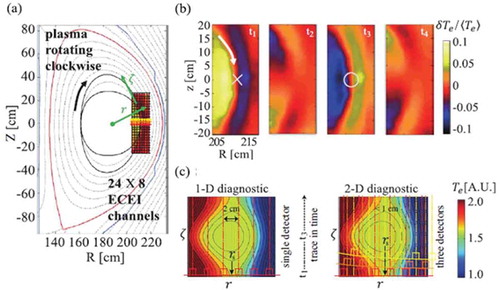
Figure 18. Parametric dependence of χ² from (a) 1-D data fit (black) and (b) 2-D data fit (red) is shown and small χ² parameter sets are used to evaluate Δ’ and ω_c for comparison. (c) Distribution of r_sΔ’ and ω_c from 1-D data (black) and 2-D data (red) shows that 2-D data set has better confidence intervals in both parameters.

Source: Choi, M.J, et al Nucl. Fusion 54, 083010, 2014., Figure 4

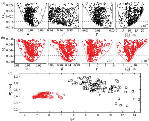
Figure 19. (a) The measured 2-D image of the 2/1 island induced by RMP is shown with the flattened T_e profile inside the island. Separatrix with X and O points is shown in purple dotted lines and flattened T_e profile is supported by the measured T_e profile with 1-D ECE. (b) Examples of cross coherence of the T_e fluctuation obtained using pairs of vertically adjacent ECEI channels inside the island, inner side and outer side of the 2/1 island are shown together with the summed coherence 2-D image. The fluctuation level is higher at X-point than at O-point. (c) The cross phase between two vertically adjacent ECEi channels measured inner and outer regions of the 2/1 island is shown. The 2-D pattern velocity is measured using the coherent cross phase. The observed flow is stronger near the O-point than that of the X-point.

Source: Choi, M.J., et al Nucl. Fusion 57, 126,058, 2017, Figure 2, Figure 3, and Figure 5

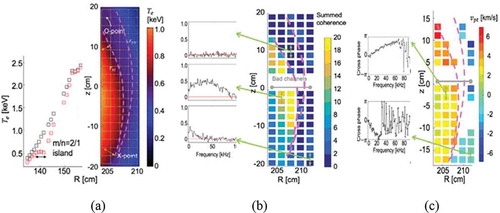
Figure 20. a) The perturbed equilibrium potential calculated from XGC1 code in presence of the 2/1 island (b) the contours of micro-instabilities (TEM and ITG) around the magnetic island in the outer mid-plane are shown, and (c) comparison of the ExB shearing rates at the O- and X-point of the magnetic island and the growth rates of the micro-instabilities are illustrated. These results are consistent with the experimental results.

Source: Kwon, J-M. et al Phys. of Plasma, 25, 052506, 2018

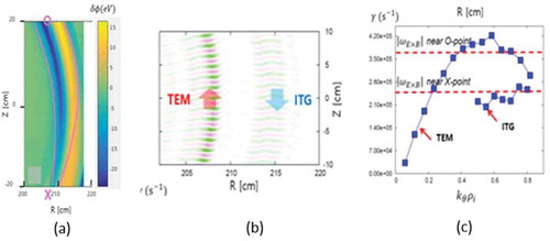
Figure 21. (a) Radial eigenmode structures for the RSAE are captured with the ECEi system on ASDEX-U. 2-D mode structure for two different times shows different toroidal mode numbers. (b) The measured RSAE on DIII-D is quite similar to those in ASDEX-U and is compared to simulated mode structures obtained with the ideal MHD code, NOVA. The improved 2-D image of the RSAE revealed shearing of the Alfvén eigenmode structure which cannot be described by NOVA. The fluctuation phase reveals an outward spiraling is well represented in the non-perturbative code, TAE/FL, where the effect of fast-ion dynamics is included in the 2-D eigenmode structure. Difference in frequency is due to omission of compressibility in modeling.

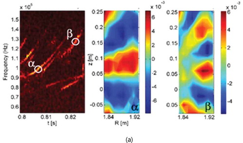
Figure 21. (a) Classen, I.G.J., et al Plasma Phys. Control. Fusion 53, 124,018, 2011. (b) Tobias, B., et al Phys. Rev. Lett. 106, 075003, 2011.

Figure 22. (a) The H-mode plasma with high edge pedestal formed by the transport barrier is shown with the cross-section of the plasma with divertor where the heat from ‘ELM’ follows the magnetic field lines. (b) Due to burst of ‘ELM’, the edge pressure/current gradients are reduced and loss of the core plasma energy is followed during ‘ELM’ event. After ‘ELM’ event, pressure/current profile recover.

Source: Conner, J.W. www.ccfe.ac.uk/assets/Documents/AIPCONFPROC103p174.pdf

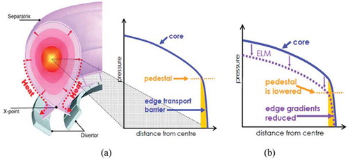
Figure 23. Schematic presentation of the peeling-ballooning mode model: as the plasma edge pressure is increased with the heating power, the point is moving along the blue arrow (α-axis) until it reaches the ballooning boundary. Then slowly increasing current moves the point along the ballooning boundary (red line). As it hits the peeling-ballooning limit, crash occurs and loses edge pressure and returns to the initial position (green line).

Source: Conner, J.W. www.ccfe.ac.uk/assets/Documents/AIPCONFPROC103p174.pdf

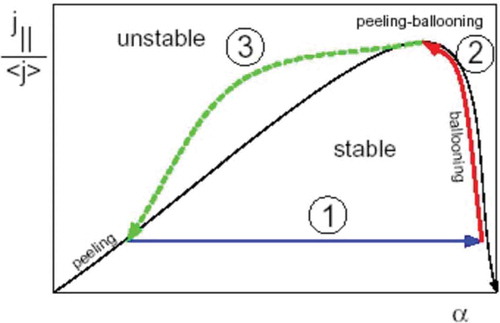
Figure 24. The filamentary structures captured by the fast camera with high toroidal mode numbers in MAST. The fast camera image is the image of the D_α light from interaction between radially moving filament structure and neutrals in the outside of the separatrix. The filamentary structure exists in the (a) inter-ELM-crash period, (b) L-mode phase, and (c) ELM-crash phase. The intensity of the mode is plotted on the toroidal plane and mode number moves from high to low as the intensity of the filament is increased.

Source: Ayed, N. B. et al, Plasma Phys. control. Fusion, 51, 035016, 2009

Figure 25. (a) The position of the ECEi window (black box) and sight of the D_α light (green line) are depicted on the calculated equilibrium flux surface. The separatrix (or last closed flux line) is in red line. (b) The captured image of the ELM with n = 8 is shown with the separatrix (red line). (c, d) D_α spikes shown together with the spectrogram of one of the ECEi channels. The arrow sign in (d) indicates the time when the image was taken.

Source: Kim, M. et al Nucl. Fusion 54, 093004, 2014

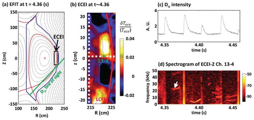
Figure 26. Identification of the measured ELM with synthetic image of the simulated edge localized eigenmode by (BOUT++). (a) Calculated eigenmode with n = 8 for the plasma equilibrium is shown, (b) Synthetic ECEi image is shown with the mirror image of down shifted spectra, (c) Background noise of the ECEi system is added, (d) The measured image of the ELM to be compared with (c).

Source: Kim, M. et al Nucl. Fusion 54, 093004, 2014

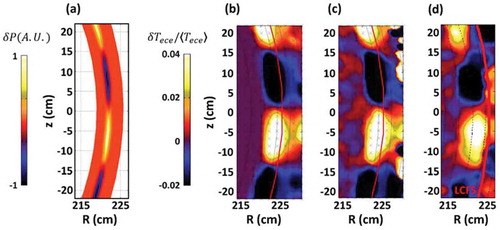
Figure 27. (a) Simultaneous emergence and growth of multiple ELM filaments (shot no. 4431) in a rotating system in counterclockwise direction (white arrows). The arrows follow the same filament illustrating the counterclockwise rotation. Multiple bursts of the same filament in a large ELM crash event indicated in the time trace of ECEi. (b) First in the series of four bursts. Bottom left sketch depicts the flux surface with filamentary perturbations and the burst zone entering the ECEi view (yellow). The white box arrow indicates the flow velocity of the filaments. (c) Third burst of the same filament, 150 μs later. The sketch above is the corresponding model. In each example, the bursting filament develops a narrow fingerlike structure bulging outward.

Source: Yun, G., Phys. Rev. Lett., 107, 045004 (2011)

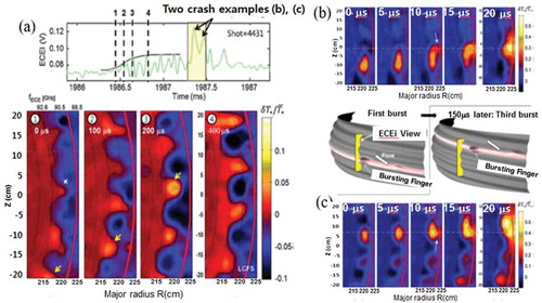
Figure 28. Observation of the ELM at both high and low field side of the plasma. The position of windows is depicted on the KSTAR geometry. The intensity of the ELM at both sides is similar and this is inconsistent with the ballooning mode model. The mode number is not consistent with the global ELM structure (white line is the same mode structure at high and low field side). Rotation direction is opposite each other with different speed.

Source: Park, H

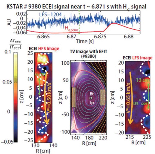
Figure 29. (a) The time trace of the fast RMP current ramp up plotted with the D_α light. 2-D images of the ELM before, middle and after the RMP current ramp up during the ELM-crash suppression experiment are illustrated. After suppression, the toroidal mode number is shifted from n ~ 15 to n ~ 20 and the ELM become marginally stable. (b) The time traces of the slowly decreasing integrated spectral powers of the ELM (blue; 5–30 kHz) and slowly increasing turbulence level (red; 30–70 kHz) along with the RMP coil current (gold) are shown.

Source: Lee, J. et al Phys. Rev. Lett. 117, 075001 2016

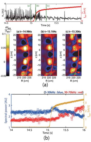
Figure 30. The ELM-crash suppression experiment with a slow RMP current ramp up and down time scale (green) comparable to the magnetic diffusion time scale (~2s) for the KSTAR edge plasma parameters. (a) The intensity of D_α spikes is linearly reduced as the amplitude of the broadband turbulence is linearly increased with the RMP current ramp up while the perpendicular flow speed of the turbulence suddenly dropped to minimum at about the same time when the ELM-crash is suppressed. The decay of the turbulence level is significantly delayed as the RMP ramp down is started and D_α spikes returned when the amplitude of turbulence dropped to the level where the suppression was started and the perpendicular rotation is increased suddenly. (b) The coherence spectra for poloidal grows as the RMP is ramped up and radial spread of the turbulence occurs when the turbulence level is fully saturated poloidally.

Source: Park, H

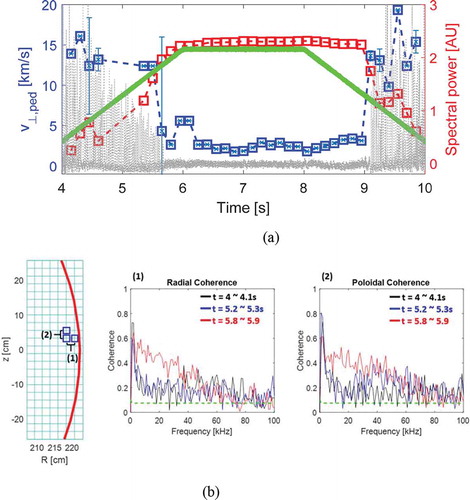
Figure 31. Simulation set up and kinking of the magnetic flux rope in solar flare. Modeling of the flux rope and development of the kink instability using ideal MHD code with the β = 0 plasma is given. The flux rope (half torus) is induced by the current under the chromosphere and the rope has driven current for the kink. This is quite similar to the case of kink instability demonstrated in sawtooth instability without boundary.

Source: Titov, V. S., Démoulin, P., Astron. Astrophys. 351, 707, 1999